Introduction
The earth is complex and dynamic, with many processes occurring beneath, in, and above the crust. Geomorphological processes such as weathering and erosion determine the surface features. Geomorphological diversity refers to the natural range of geological, geomorphological, and soil features, processes currently acting on rocks, landforms, soils, and topography of a defined area (Kori et al. 2019; Kot 2018; Panizza 2009). Geomorphodiversity, which falls within the broad geosciences field of geodiversity, is a critical and specific assessment of forms or surface features of a defined place on Earth (Kori et al. 2019; Panizza 2009). Geomorphodiversity cannot be univocal, having extrinsic and intrinsic aspects (Panizza 2009). Extrinsic factors are morphostructural, morphoclimatic, morphographic, morphogenetic, and morphometric characteristics, and intrinsic aspects include the diversity and complexity of landforms, assessing the total range of phenomena, and comparing them to each other. Both approaches, whether individually or combined, start with a geomorphological map (Panizza 2009).
An intrinsic and extrinsic diversity assessment explains why the environment is characterized by an interaction of rocks, water, air, and humans. This geomorphodiversity study critically and specifically assesses the geomorphological features of Komati Gorge by comparing them intrinsically and extrinsically. The geomorphological features are then mapped to visualize the characteristics and behavior of the morphology of the area, the morpho-characteristics of the Komati Gorge. The study is based on the identification of geomorphological elements that independently characterize the landscape of a terrain (Panizza 2011).
Materials and Methods
Study Area
The study was conducted in the Komati Gorge (Fig. 1), a river valley situated in the northeastern part of South Africa, near the communities of Carolina and Machadodorp in Mpumalanga Province. Komati Gorge is in the upper reaches of the perennial Komati River, situated at latitude 25o 52' 4,19" S and longitude 30o 18' 15,60" E.
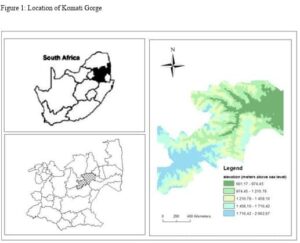
Figure 1. Location of the study area, Komati gorge
The Komati River originates from the Transvaal plateau near Breyton in the Drakensberg range west of the small-town Carolina in the Mpumalanga Province in South Africa (Mahlathi 2018; Nkomo and van der Zaag 2004). It flows into Swaziland and then re-enters South Africa where it is joined by the Crocodile River at the border with Mozambique to form the Incomati basin. The Incomati River then flows north-eastwards to the Indian Ocean at Maputo Bay in Mozambique (Nkomo and van der Zaag 2004). The Komati River is approximately 480 km long from its source to the confluence with the Crocodile River. The total catchment area of the Komati River is approximately 50,000 km2 (Nkomo and van der Zaag 2004).
From upstream to downstream, the Incomati basin comprises Precambrian granites and gneiss of the Archean, and Cretaceous and Karroo lavas of the Mesozoic (Romano 1965). The area is dominated by wide sandstone krantzes, with exposures of the Kromberg Formation and upper Hooggenoeg Formation of the Onverwacht Series (Dann 2000). It also consists of a riparian zone, bluff habitat, thorn bushveld, and Highveld grassland.
Data and Sources
Relevant factors for the assessment of geomorphological diversity of the Komati Gorge were selected following the definition of geodiversity. The topographic Position Index (TPI), Topographic Wetness Index (TWI), and insolation are relevant choices for geodiversity assessment (Najwer and Zwoliński 2014). Geology, soil, relative height, erodibility, ruggedness, and land use/land cover were then selected based on their correlation with the first three factors. The eight factors can characterize geodiversity in the fullest possible way (IAG/AIG 2019; Kori et al. 2019).
Geomorphometric parameters, namely soil erodibility, development ratio, drainage density, drainage texture, stream length ratio, and ruggedness were calculated using mathematical formulae 1 to 6. The mathematical formulae were used in combination with the 30-m raster size SRTM DEM (Digital Elevation Model) aerial photographs (Price et al. 2011). The photographs were obtained from National GeoSpatial Information (NGI) and data extracted using System for Automated Geoscientific Analysis Geographic Information System (SAGA GIS), Environmental System Research Institute Aeronautical Reconnaissance Coverage Geographic Information System (Esri ArcGIS) 10.2, and Esri ArcGIS Pro 1.2. The SRTM downloader tool in the ArcGIS 10.2 map server was used to download the 30-m raster size SRTM DEM from the NGI.
A 30 arc-second raster size Harmonized World Soil Database layer was obtained from the International Institute for Applied Systems Analysis (IIAS) online database. The erodibility of the soil was obtained from calculating the soil erodibility factor (K factor) using the Bouyoucos method (Bouyoucos 1935). This method was chosen for its ability to efficiently match field data in addition to its simplicity to use in GIS (Kori et al. 2019). The erodibility of the soil accounts for the influence of the intrinsic soil properties (Wang et al. 2001). The intrinsic soil properties may characterize and serve as an indicator for soil taxonomy (Svoray and Shoshany 2004). The intrinsic soil factors affect and are also affected by the variations in soil properties. Soil erodibility is used in quantifying geomorphic diversity because it significantly influences landform and landscape development (Kori et al. 2019).
Geological data was downloaded from the South African Geosciences online database. Hydrography systems shapefiles were obtained from the Department of Water Affairs and Forestry (DWAF). Land use/land cover shapefiles for 2020 were obtained from the
Department of Rural Development and Land Reform (DALRRD).
Creation of Factor Maps
The geologic, hydrologic, soil and land use/land cover data were analyzed using SAGA GIS, ArcGIS 10.2, and ArcGIS Pro. The hydrography factor map is the result of the addition of three maps showing the diversity of rivers, lakes, and the TWI. The TWI map was created from DEM in terrain analysis tools (hydrology) in SAGA GIS. It was based on a modified catchment area calculation which does not think of the flow as a very thin film (IAG/AIG 2019; Kori et al. 2019). The lakes were assessed based on shoreline Development Ratio (DL) (Minár et al. 2005) computed using formula 1. Calculations were done in an attribute table of the hydrography layer in ArcMap. Rivers were assessed using the average slope at about 100 m long. The tool for creating points on lines in ArcMap was used to divide the rivers into 100 m sections.
𝐷𝐿 = 𝐿 2 √𝜋𝐴 1.
where DL = Shoreline Development Ratio; L = Length; 𝜋 = 3.14; A = Area.
The geology factor map was created in ArcMap from the geology shapefiles. Lithological diversity information was extracted from the attribute table (Table 1) of the geology shapefile and combined with the rock hardness using the raster calculator of ArcMap to produce the final geology factor map. The geology shapefiles provided attributes of each polygon, which indicated the presence of a dominant rock type and the presence of other rocks. The soil factor map was produced in ArcMap based on the topsoil erodibility (K) factor from the obtained soil layers. The topsoil was considered because it is more sensitive to erosion. The (K) factor was calculated using a formula by Bouyoucos (Bouyoucos 1935) method.
Erodibility (K) = [(sand + silt) / (clay)] / 100 2.
Table 1. Soil erodibility
Soil type (%) | Total sand (%) | Total silt (%) | Total clay (%) | Erodibility (k) |
Lithic Leptosols | 06 | 92 | 02 | 0.49 |
Rhodic Lixisols | 21 | 67 | 12 | 0.07 |
Rhodic Acrisols | 13 | 83 | 04 | 0.24 |
Dystric and Eutric Regosols | 10 | 67 | 23 | 0.03 |
Rhodic nitisols | 19 | 76 | 05 | 0.19 |
Rhodic ferrallisols | 18 | 69 | 13 | 0.06 |
The erodibility layer was then added to the soil layer to produce the soil factor map. Producing a map based on soil erodibility (K) is important because of the intrinsic characteristics of a soil to be eroded (Kori et al. 2019; Oparaku et al. 2016).
The land use/land cover factor map was created based on the expert classification in ArcGIS Pro 1.2 from the downloaded shapefiles. The geomorphodiversity analysis of hydrological, geological, soil, and land use/land cover data was done by overlaying appropriate hydrological, geological, soil, and land use/land cover maps as thematic maps to a shaded relief to achieve composite visualization. This was to get morphographic, morphometric, structural, and morphogenetic data of features. The visualization of topographic attributes and their analysis is a useful tool for understanding the geomorphological features and processes acting on them. The first three maps were then reclassified into five geodiversity classes using Jenks’ natural breaks classification method in spatial analyst tools (reclass) in ArcMap and land use/land cover in ArcGIS Pro and saved (Jenks 1967).
Insolation was calculated in both SAGA GIS and ArcGIS Pro 1.2. In SAGA using terrain analysis tools (lightning), the DEM was automatically analyzed to get the map for the analysis area for the whole year. Ruggedness was computed using the topographic roughness index in SAGA GIS. The roughness factor expresses the amount of elevation difference between adjacent cells of a DEM (Kori et al. 2019). The landscape roughness is a measure of the irregularities of a topographic surface.
The slope position factor map classifies the landscape into cliffs, scree slopes, transportation mid-slopes, foot slopes, and open valleys (Kori et al. 2019). A slope position map was obtained from the DEM using TPI in raster tools in QGIS. The TPI was chosen for slope analysis because it is the difference between a cell elevation value and the average elevation of a neighboring area around the cell (De Reu et al. 2013). The TPI was computed considering a 300-m radius circle neighborhood in tandem with the 30-m resolution of the DEM.
Relative height is a measure of the elevation of a place in its surroundings. It shows the diversity of local heights, which reflects the energy of the relief and is a measure of elevation of a place. DEM was used to show the diversity of relative heights, which reflects the energy of the relief (Zwoliński 2008; Zwoliński 2009). The values were calculated for each grid cell using the spatial analyst tools to analyze the neighborhood (Focal Statistics) in a 3 × 3 grid cells moving window in ArcMap.
The drainage texture parameters describe the characteristics of the basin including the length of overland flow, constant of channel maintenance, frequency, drainage density, drainage texture, infiltration number, and intensity of the drainage network (Biswas 2016; Chethan and Vishnu 2018). Drainage texture is classified according to standard metrics (Table 2). The drainage density is the ratio of the total length of streams of all orders to the area of the basin. The value range of the drainage density is approximately a minimum of 0 and a maximum of 5000 m-1. It is calculated for all the river channels and interpreted according to the type of landscape. Drainage density is given by:
Dd = L / A 3.
where Dd = Drainage density; A = Area of basin; L = Total length of the stream.
Table 2. Five classes of drainage texture (Source: (Magesh et al. 2013))
Very coarse | <2 |
Coarse | 2 to 4 |
Moderate | 4 to 10 |
Fine | 10 to 15 |
Very fine | >15 |
The relative height factor map in raster format was added to ArcMap and standardized into five geodiversity classes using Jenks’ natural breaks classification method (Jenks 1967) in spatial analyst tools (reclass) and saved. Insolation and ruggedness factor maps in raster format were added to ArcGIS Pro and standardized into five geodiversity classes using Jenks’ natural breaks classification method (Jenks 1967) in spatial analyst tools (reclass) and saved. Jenks natural breaks classification method is a data classification method designed to optimize the arrangement of a set of values into "natural" classes. This method seeks to minimize the average deviation from the class meanwhile maximizing the deviation from the means of the other groups. The features are divided into classes whose boundaries were set where there are relatively big differences in the data values. It is also known as the goodness of variance fit (GVF), which is equal to the subtraction of the sum of Squared Deviations for Class Means (SDCM) from the sum of Squared Deviations for Array Mean (SDAM). The slope positions factor map was reclassified into five geodiversity classes by the table in the processing toolbox (raster analysis) in QGIS and saved.
The Final Geomorphological Map
The geomorphological map is the most prominent output from this study. The eight-factor maps were combined as raster layers to produce a geomorphological map. Before overlaying the eight factors, the Multi-Criteria Evaluation (MCE) using the Analytic Hierarchy Process (AHP) criteria were employed to calculate relative weights for each factor map (IAG/AIG 2019). Table 3 shows the ranking values of each factor in percentage. The AHP applies a pairwise comparison to provide a basis for the criteria used in decision analysis and determines values for each of the criteria (Cay and Uyan 2013). A matrix is then generated because of pairwise comparisons and criteria weights are reached because of the calculations. The ordered weighted averaging tool from grid analysis in processing tools in QGIS was used to combine the factor maps. Geomorphological characteristics of the factor maps were added as tabular attribute information linked to the vector information as attribute data.
Table 3. Geomorphological factor ranking values
Category | Values (%) |
| Rank |
Relative height |
| 17,2 | 3 |
Insolation |
| 3,6 | 6 |
Hydrography |
| 37 | 1 |
Geology |
| 7,7 | 4 |
Soil |
| 1,8 | 8 |
Ruggedness |
| 25,1 | 2 |
Slope positions |
| 4,2 | 5 |
Land use/land cover |
| 3,3 | 7 |
Results and Discussion
Factor maps
The hydrography factor reveals the interplay of high elevation areas, waterways, and open valleys. Low hydrography occupies 50% of Komati Gorge, revealing that Komati Gorge has few surface water resources (Fig. 2). There are large areas of hard and very hard rocks (Fig. 3; Table 4) because the area is rich in rocks such as sandstones, cherts, and basaltic rocks. Geology affects soils and waterways. Rock hardness (Table 4) indicates density and resistance to breaking. The hardness and strength of the rocks are necessary parameters in this study as they are a function of the individual rock type. The hard, impermeable rock types resist rivers in the Komati Gorge to create many water paths and cut deep, which means that the water bodies of this area are mainly shallow.
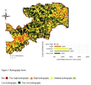
Figure 2. Komati Gorge hydrography factor map
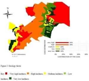
Figure 3. Komati Gorge geology factor map
Table 4. Rocks found in Komati Gorge
Main rock type | Rock Names | Hardness of the main rock (Mohs) | Combined lithological diversity and rock hardness |
Sedimentary | Amygdaloid intermediate lava, tuff, quartzite, shale, conglomerate | 3 | 8 |
Igneous | Tuff, agglomerate and basalt | 5 | 8 |
Igneous | Medium to coarse-grained, homogeneous hornblende and hornblende biotite tonalite | 6 | 9 |
Igneous | Biotite trondhjemite gneiss | 7 | 8 |
Igneous | Ultramafic to felsic lavas and pyroclastic rocks | 5 | 7 |
Sedimentary | Dolomite, Subordinate chert, Carbonaceous shale, limestone and Quartzite | 6 | 10 |
Sedimentary | Quartzite, subordinate Conglomerate and shale | 5 | 8 |
Sedimentary | Shale, limestone/dolomite, basalt and tuff | 5 | 9 |
Igneous | Diabase | 7 | 8 |
Igneous | Andesite and conglomerate | 7 | 9 |
Sedimentary | Shale, quartzite, conglomerate, breccia and diamictite | 4 | 9 |
Igneous | Ultrabasic rocks | 5 | 6 |
metamorphic | Coarse-grained, porphyritic granodiorite/adamellite, gneiss and migmatite | 6 | 10 |
Sedimentary | Quartzite, siltstone, conglomerate, shale and andesite | 6 | 11 |
The soil factor map (Fig. 4) shows that Komati Gorge has highly erodible soils. About 17 % of the soils have low credibility and occupy the south section of the gorge only. Soil factors affect other factors such as river networks and slope angles, which are directly influenced by soil erodibility. Rivers follow easily erodible terrain while highly erodible soils create plains. Slopes and river channels in the Komati Gorge conform to this general anticipation. The land use/land cover factor map (Fig. 5) reveals how and what the land in Komati Gorge is used for. The map shows that much of the land (over 90%) is used for either one of the uses in Table 5. The land use/land cover map strongly corresponds with the relative heights, hydrography, soil, and insolation.
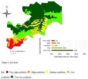
Figure 4. Komati Gorge soil factor map
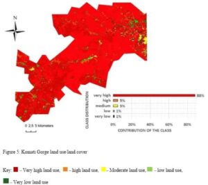
Figure 5. Komati Gorge land use/land cover factor map
Table 5. Komati Gorge land use/land cover
Land uses/land cover | Expert classification |
Indigenous forest | Forested land |
Low forest thicket | Forested land |
Dense and open-sparse plantation forest | Forested land |
Woodland | Forested land |
Temporary unplanted (clear-felled) | Forested land |
Low shrubland | Shrubland |
Sparsely wooded grassland | Grassland |
Natural grassland | Grassland |
Dry pans | Barren land |
Flooded pans | Water bodies |
Rivers | Water bodies |
Artificial dams | Water bodies |
Herbaceous wetlands | Wetlands |
Natural rock surfaces | Barren land |
Eroded lands | Barren land |
Bare riverbed material and other bare | Barren land |
Cultivated commercial permanent orchards | Permanent crops |
Sugarcane non-pivot | Permanent crops |
Commercial annual crops pivot irrigated and non-irrigated | Cultivated |
Rain-fed/dry land | Cultivated |
Fallow land-old fields | Cultivated |
Residential formal and informal | Built-up |
Village scattered and dense | Built-up |
Smallholdings | Built-up |
Urban recreational fields | Built-up |
Commercial | Built-up |
Industrial | Built-up |
Roads-rails (major-linear) | Built-up |
Mines | Mines and quarries |
Surface infrastructure | Mines and quarries |
Extraction pits | Mines and quarries |
Quarries | Mines and quarries |
Tailings | Mines and quarries |
Resource dumps | Mines and quarries |
The relative height factor map (Fig. 6) reveals the interplay of many factors and the dominance of rough surfaces such as mountains, hills, cliffs, and open valleys, an indicator of high local differences in elevation between cells. The high diversity of local heights reveals the high energy of the relief of Komati Gorge. This factor affects other factors such as the ruggedness of the area, which decreases with an increase in elevation. Over 90 % of Komati Gorge experiences high to very high insolation (Fig. 7). Since the area is dominated by high-lying areas, it can be concluded that these are the ones receiving such high insolation, and the remaining 6 % low-lying areas would receive less insolation. This may be due to the shading effect of the high elevation areas. The insolation factor directly affects other factors such as soil, geology, and hydrology. The soil of the high-lying areas is more substantially developed than soils in low-lying areas. Rocks in areas of high insolation are rich in iron.
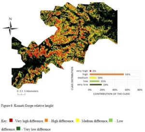
Figure 6. Komati Gorge relative height factor map
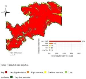
Figure 7. Komati Gorge insolation factor map
Over 70% of Komati Gorge has low ruggedness (Fig. 8), namely areas at high elevations. Only 25 % is found at low elevations with high ruggedness, along the mountain edges and river valleys. The ruggedness factor strongly correlates with slope position and relative height factors. The uneven distribution of river valleys and cliffs is clear (Fig. 9). Slope positions further classify the landscape into five morphological classes.
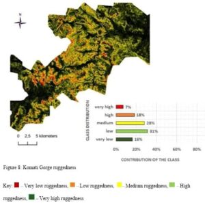
Figure 8. Komati Gorge ruggedness factor map
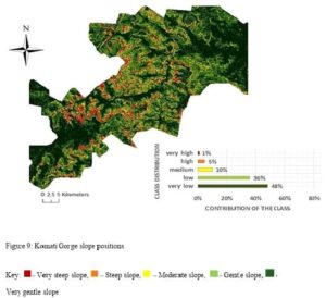
Figure 9. Komati Gorge slope positions factor map
The final geomorphodiversity map (Fig. 10) reveals the variable influence of different factors on the geomorphology of Komati Gorge. The edges of the area have very high geomorphodiversity while the inner part has very low geomorphodiversity. Over 70% of the area has medium to very high and 21% has low geomorphodiversity. The area of high geomorphodiversity is based on over 90% of different land uses. These areas are located at high elevations, receive 94 % of insolation and constitute valleys and rivers. They also had highly erodible soil, and very negligible (2 %) ruggedness.
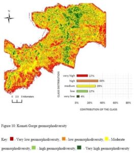
Figure 10. The variable influence of different factors on the geomorphology of Komati Gorge
Concluding Remarks
Geomorphological mapping, a now flourishing science, provides a firm basis for the investigation of geomorphological features. The geomorphological map produced provides insights into geological processes that shaped the Gorge. The map revealed that the southwest parts of Komati Gorge have high geomorphological diversity. The northeast parts of Komati Gorge have low to medium geomorphological diversity. Hydrography, ruggedness, relative heights, and geology carried more weight and had the most noticeable influence on the geomorphological diversity of Komati Gorge. Slope position, soil erodibility, insolation, and land use/land cover carried the least weight and were observed as minor influencers of the geomorphological diversity of Komati Gorge.
Acknowledgments
Mudau Mukhodeni wishes to acknowledge the Department of Ecology and Resources Management. I would like to thank my supervisor, Mr E. Kori, for his good communication, providing a good learning environment, and for guiding me throughout my learning experience.
Author contributions
Mudau Mukhodeni drafted the paper and did the GIS extractions and calculations. Edmore Kori corrected and proofread the paper before submission.