Department of Mathematics, Kurukshetra University, Haryana, 136 119, IN
Department of Mathematics, National Institute of Technology, Haryana, 136 119, IN
Abstract
Purpose
The purpose of this paper is to study the reflection of plane periodic wave’s incident on the surface of generalized thermoelastic micropolar transversely isotropic medium.
Methods
Plane wave propagation is studied to calculate complex velocities of the four waves from the complex roots of a quartic equation. The complex velocity of the attenuated wave in the medium is resolved to calculate its propagation (phase) velocity and quality factor of attenuation. Reflection of waves at the free surface of micropolar transversely isotropic generalized thermoelastic elastic half-space has been discussed.
Results
Numerical examples calculate the amplitude ratios of reflected waves at the free surface of the micropolar transversely isotropic generalized thermoelastic elastic half-space to evince the effects of anisotropy and theories of generalized thermoelasticity.
Conclusions
It is concluded from the present study that there are four quasi wave propagates in of generalized thermoelastic micropolar transversely isotropic medium viz., quasi-longitudinal displacement (qLD) wave, quasi-transverse displacement (qTD) wave, quasi- transverse microrotational (qTM) wave and quasi thermal (qT) waves.
Background
Depending upon the mechanical properties, the material of the earth has been classified as elastic, viscoelastic, sandy, granular, microstructure, etc. Some parts of the earth may supposed to be composed of material possessing micropolar/granular structure instead of continuous elastic material.
To explain the fundamental departure of microcontinuum theories from the classical continuum theory, the former is a continuum model embedded with microstructures to describe the microscopic motion or a non-local model to describe the long-range material interaction. This extends the application of the continuum model to microscopic space and short-time scale. Micromorphic theory [
1
,
2
] treats a material body as a continuous collection of a large number of deformable particles, with each particle possessing finite size and inner structure. Using assumptions such as infinitesimal deformation and slow motion, micromorphic theory can be reduced to Mindlin’s microstructure theory (1964). When the microstructure of the material is considered rigid, it becomes the micropolar theory [
3
].
Eringen’s micropolar theory is more appropriate for geological materials like rocks and soil since this theory takes into account the intrinsic rotation and predicts the behavior of material with inner structure. The linear theory of micropolar thermoelasticity was developed by [
4
] and [
5
] to include thermal effects and is known as micropolar coupled thermoelasticity.
Inspite of these studies, no attempt has been made to study the reflection of waves in transversely isotropic micropolar generalized thermoelastic medium. Thus, the present study of the effect of anisotropy in a reflection of waves at the free surface of transversely isotropic micropolar generalized thermoelastic medium has its due importance in engineering and geophysical problems where the situation so demands.
We analyze the reflection of waves in transversely isotropic micropolar generalized thermoelastic medium. This study has many applications in various field of science and technology, namely, atomic physics, industrial engineering, thermal power plants, submarine structures, pressure vessel, aerospace, chemical pipes and metallurgy.
Basic equations
The basic equations in dynamic theory of the plain strain of a homogeneous and micropolar transversely isotropic generalized thermoelastic solid in the absence of body forces, body couples and heat sources are given by the following:
where
tkl,mkl,
and
Kkl
are the stress tensor, couple stress tensor and thermal conductivity tensor, respectively;
qk
is the heat flux vector;
η
is the entropy;
T
is the absolute temperature;
C∗
is the specific heat at constant strain;
τ0
and
τ1
are the thermal relaxation times;
ρ
is the bulk mass density;
횥
is the microinertia;
ul
and
ϕk
are the components of displacement vector and microrotation vector, respectively;
βkl
is the thermal elastic coupling tensor;
Aklmn,Gklmn,Blkmn
are characteristic constants of material where
Aklmn,Blkmn
satisfies the symmetric properties
Aklmn=Amnkl,Bmnlk=Blkmn,
and
βkl=βlk
and
Kkl=Klk
. Tensor
Gklmn
does not possess this property; it forms a pseudo-tensor, inversion of the coordinate system changing its sign. In a centrosymmetric body, all components of
Gklmn
vanish.
Formulation of the problem
We have used appropriate transformations following [
6
] on the set of Equations
1
to
5
to derive equations for micropolar thermoelastic transversely isotopic medium and restricted our analysis to the two-dimensional problem.
We consider a homogeneous, centrosymmetric, micro polar thermoelastic transversely isotropic medium initially in an undeformed state and at uniform temperature
To
. We take the origin of coordinate system on the top plane surface and
x3
-axis pointing normally into the half-space, which is thus represented by
x3≥0
. We consider plane waves such that all particles on a line parallel to
x2
-axis are equally displaced, so all partial derivatives with respect to the variable
x2
would be zero. Therefore, we take
u→=(u1,0,u3),ϕ→=(0,ϕ2,0)
and
∂/∂x2=0
so that the field equations and constitutive relations reduce to the following:
A11∂2u1∂x12+A13+A56∂2u3∂x1x3+A55∂2u1∂x32+K1∂ϕ2∂x3−β11+τ1∂∂t∂T∂x1=ρ∂2u1∂t2,A66∂2u3∂x12+A13+A56∂2u1∂x1x3+A33∂2u3∂x32+K2∂ϕ2∂x1−β31+τ1∂∂t∂T∂x3=ρ∂2u3∂t2,B77∂2ϕ2∂x12+B66∂2ϕ2∂x32−Xϕ2+K1∂u1∂x3+K2∂u3∂x1=ρ횥∂2ϕ2∂t2,K1∗∂2T∂x12+K3∗∂2T∂x32=ρC∗∂∂t+τo∂2∂t2T+To∂∂t+noτo∂2∂t2×β1∂u1∂x1+β3∂u2∂x2.t33=A13∂u1∂x1+A33∂u3∂x3−β3(1+τ1∂∂t)T,t31=A65∂u3∂x1+K1ϕ2+A55∂u1∂x3,m32=B66∂ϕ2∂x3,
where
β1=A11α1+A13α3,β3=A31α1+A33α3,K1=A56−A55,K2=A66−A56,X=K2−K1,α1,α3
are the coefficients of linear thermal expansion, we have used the notations
11→1,33→3,12→7,13→6,23→5
for the material constants.
For L-S theory
τ1=0no=1
; for G-L theory,
τ1>0no=0
; and for coupled thermoelasticity theory,
no=0,τ1=τo=0
. The thermal relaxation times
τ0
and
τ1
satisfy the inequality
τ1≥τ0>0
for G-L theory only. However, it has been proved by [
7
] that the inequalities are not mandatory for
τ0
and
τ1
to follow.
For further considerations, it is convenient to introduce the dimensionless variables defined by the following:
x1′=ω∗c1x1,x3′=ω∗c1x3,u1′=ω∗c1u1,u3′=ω∗c1u3,ϕ2′=A55K1ϕ2,tij′=tijA11,mij′=mijc1B56ω∗,T′=TTo,t′=ω∗t,τo′=ω∗τo,τ1′=ω∗τ1,ω∗2=Xρ횥,c12=A11ρ,
where
ω∗
is the characteristic frequency of the material, and
c1
is the longitudinal wave velocity of the medium.
Plane-wave propagation
Let
p→(p1,0,p3)
denotes the unit propagation vector,
c
and
k
are the phase velocity and the wave number of the plane waves propagating in
x1x3
plane, respectively. We seek plane-wave solution of the equations of motion of the form
(u1,u3,ϕ2,T)=(ū1,ū3,ϕ̄2,T̄)eιξ(p1x1+p3x3−ct).
Making use of Equation
18
and the values of
u1,u3,ϕ2
and
T
from Equation
19
in the Equations
11
to
14
, we obtain four homogeneous equations in four unknowns
ū1,ū3,ϕ̄2
and
T̄
, which for the non-trivial solution yield
Ac8+Bc6+Cc4+Dc2+E=0,
where
A=b4−b5/ω2,B=g1+g6/ω2,C=g3+(g2+g4)/ω2+g4/ω4,D=g5+g7/ω2,E=g8,g1=b1−b2′−b4a1,g2=b8−b2−b4a1+b17a14+b12a15−a1b5,g3=b6′−b1−b3+b2′a1+b12′a10,g4=b6+a1b2+a10×(b12−b13′)+a14(b15−b18+b15′)−a15b18,g5=b7+b3a1+b9a10−a1b6′,g6=b5a1−a15b22,g7=b14a14+b20a15−b6a1−a10b10,g8=−b7a1−b11a10,g9=b19a15−a1b8−a10b13,b1=d7a8d12,d1=A55A11,d2=(A13+A56)A11,d3=K12A11A55,d4=A66A11,d5=A33A11,d6=K1K2A11A55,d7=B66ρ횥c12,d8=B77ρ횥c12,d9=Xρ횥ω∗2,d10=A55ρ횥ω∗2,d11=K2K1d10,d13=β3ToA11,d18=A13A11,d14=β1ToA11,d15=K1∗A55,,d16=A56A11β̄=β1β3,K̄=K1∗K3∗,ε1=ρC∗c12K3∗ω∗,ε2=β3c12K3∗ω∗.b2=d7(a8d11+d9d6)+a7a4d12,b2′=a2a9d12,b3=a8(a6d7+a2d12),b4=d12d7a9,b5=d7d11a9,b6=a6a7a4+a8(a2d11−a3a5),b6′=a2a6a9,b8=a9(a2d11−a3a5),b7=a2a6a8,b9=a8a11d12,b10=a11(a8d11+a6d9)+a5a8a12−a6a7a13,b11=a8a6a11,b12=−a7a13d12,b12′=a9a11d12,b13=a7a13d11,b13′=a9(a11d12+a5a12),b14=a8(a1a3+a2a12),b15=a7(a4a12−a3a13),b15′=a9(a1a3+a2a12),b16=a8a12d7,b17=−a9a12d7,b18=d12(a4a11+a2a13),b19=d11(a14a4+a2a13)−a6a13d7+a5(a4a11−a3a13),b20=a6(a4a11+a2a13),b21=a13d12d7,b22=a13d7d11,a1=d1p32+p12,a2=d5p32+p12d4,a3=ıp1d10,a4=p3ωε2(1−ιωτ1),a5=ıp1d6,a6=d7p32+p12d8,a7=−ıp3d14×(1−ıωτ1),a8=p32+k̄p12,a9=−ıε1×(1/ω−ıτo),a10=p1p3d2,a11=−p1p3d5,a12=ıp3d9,a13=p3ωε2p1β̄(1−ιωτ1),a14=ıp3d3,a15=−ıp1d3(1−ιωτ1).
The complex coefficient implies that four roots of this equation may be complex. The complex phase velocities of the quasi-waves, given by
ci,i=1,2,3,4
, will be varying with the direction of phase propagation. The complex velocity of a quasi-wave, i.e.
ci=cR+ıcI,
defines the phase propagation velocity
Vi=(cR2+cI2)/cR
and attenuation quality factor
Qi−1=−2cI/cR
for the corresponding wave. Therefore, four waves propagating in such a medium are attenuating. The same directions of wave propagation and attenuation vector of these waves make them homogeneous wave. These waves are called quasi-waves because polarizations may not be along the dynamic axes. The waves with velocity
Vi(i=1,2,3,4)
may be named as quasi-longitudinal displacement (qLD) wave, quasi-transverse displacement (qTD) wave, quasi-transverse microrotational (qTM) wave and quasi thermal wave (qT) that are propagating with the descending phase velocities, respectively.
Reflection at the free surface
We consider a homogeneous micropolar generalized thermoelastic transversely isotropic half-space occupying the region
x3>0
. Incident qLD or qTD or qTM or qT wave at the interface will generate reflected qLD, qTD, qTM and qT waves in the half-space
x3>0
. The total displacements, microrotation and temperature distribution are given by the following:
u1=∑j=18AjeıEj,u3=∑j=18BjeıEj,ϕ2=∑j=18CjeıEj,T=∑j=18DjeıEj,
where
Ej=ω[t−(x1sinej−x3cosej)/cj],j=1,2,3,4,Ej=ω[t−(x1sinej+x3cosej)/cj],j=5,6,7,8,
ω
is the angular frequency. Here, subscripts 1,2,3, and 4 denote the quantities corresponding to incident qLD, qTD, qTM and qT wave, respectively, whereas the subscripts 5,6,7 and 8, respectively, denote the corresponding reflected waves and
Bj=Λ1iΛiAj,Cj=Λ2iΛiAj,Dj=Λ3iΛiAj,(j=1,…,8),Λi=d7ω2−ξ2a2ξa5ξa7ξa3ω2−d11−ξ2a60ξa40a9+a8ξ2,Λ1i=ξ2a11ξa5ξa7ξa12ω2−d11−ξ2a60ξa130a9+a8ξ2,Λ2i=ξ2a11d7ω2−ξ2a2ξa7ξa12ξa30ξa13ξa4a9+a8ξ2,Λ3i=ξ2a11d7ω2−ξ2a2ξa5ξa12ξa3ω2−d11−ξ2a6ξa13ξa40.
The expressions for
ai,i=1,2,....15
are obtained from the expressions for
ai,i=1,2,....15
given in Equation
21
on substituting the values for
p1
and
p2
.
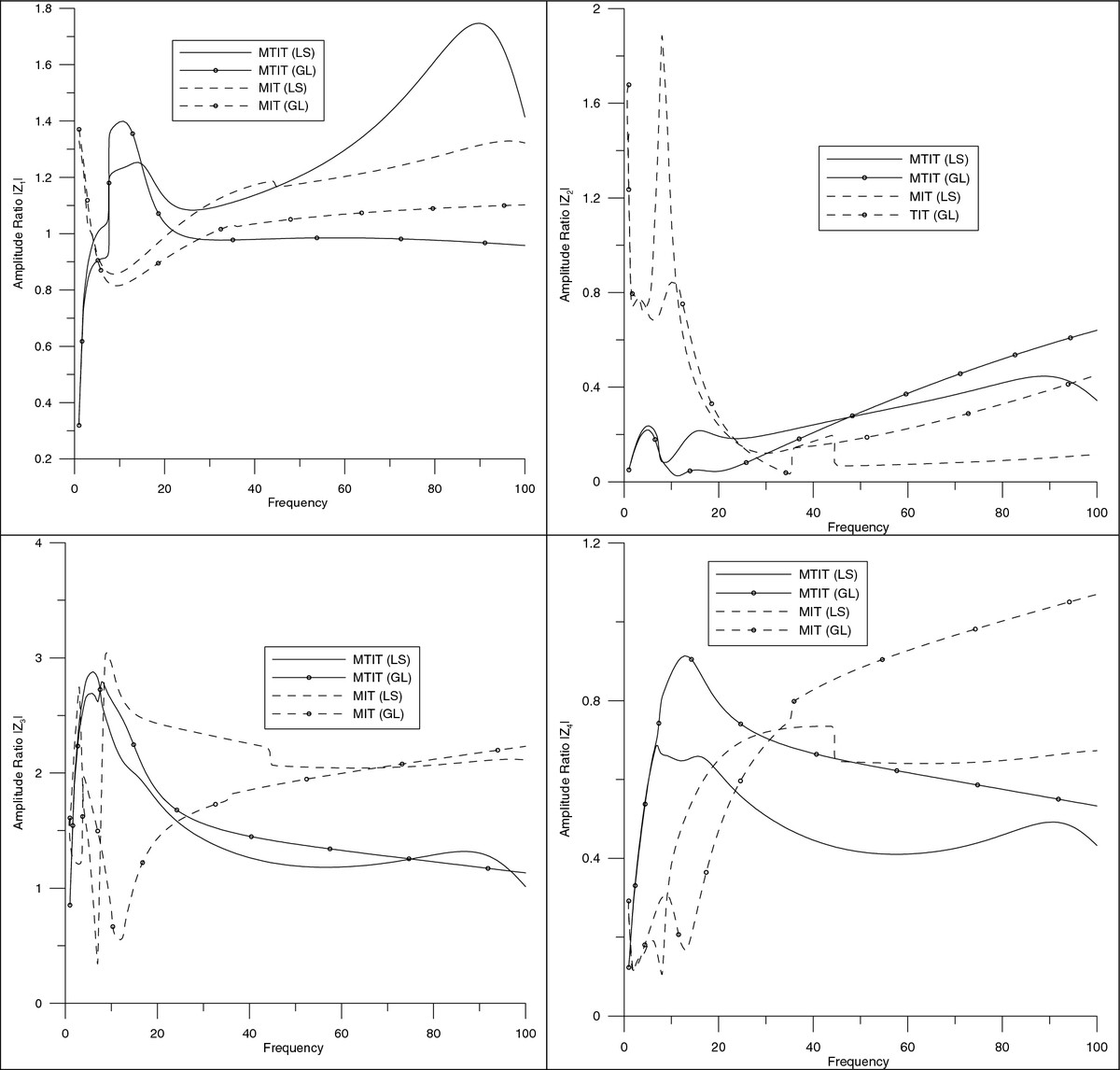
Figure 1
a)
|Z1|
b)
|Z2|
c)
|Z3|
d)
|Z4|
for incident qLD wave.
For incident qLD wave,
p1=sine1,p3=−cose1
; for incident qTD wave,
p1=sine2,p3=−cose2
; for incident qTM wave,
p1=sine3,p3=−cose3
; for incident qT wave,
p1=sine4,p3=−cose4
; for reflected qLD wave,
p1=sine5,p3=cose5
; for reflected qTD wave,
p1=sine6,p3=cose6
; for reflected qTM wave,
p1=sine7,p3=cose7
; and for reflected qT wave,
p1=sine8,p3=cose8
.
Boundary condition
We assume that the boundaries of the half-space are stress-free thermally insulated. Therefore, the appropriate boundary conditions at the surface
x3=0
are as follows:
Vanishing of the normal stress
t33=0,
Vanishing of the tangential stress
t31=0,
Vanishing of the tangential couple stress
m32=0,
Vanishing of the temperature gradient
∂T∂y+hT=0=0,
where
h
is the surface heat transfer coefficient;
Figure 2
a)
|Z1|
b)
|Z2|
c)
|Z3|
d)
|Z4|
for incident qTD wave.
h→0
corresponds to thermally insulated boundaries and
h→∞
refers to isothermal boundaries.
The boundary conditions given by Equations
27
to
30
must be satisfied for all values of
x1
and
t
, so we have
E1(x1,0,t)=E2(x1,0,t)=...................=E8(x1,0,t).
Then from Equations
23
,
24
and
31
, we have
sine1c1=sine2c2=...=sine7c7=sine8c8=1c,
which corresponds to the Snell’s law in the present case and
ξ1c1=ξ2c2=...=ξ8c8=ω.
Figure 3
a)
|Z1|
b)
|Z2|
c)
|Z3|
d)
|Z4|
for incident qTM wave.
Figure 4
a)
|Z1|
b)
|Z2|
c)
|Z3|
d)
|Z4|
for incident qT wave.
Here,
e1=e5
,
e2=e6
,
e3=e7
and
e4=e8
i.e. the angle of incidence is equal to the angle of reflection in micropolar transversely isotropic generalized thermoelastic solid so that the velocities of reflected waves are equal to their corresponding incident waves, i.e.
c1=c5
,
c2=c6
,
c3=c7
and
c4=c8
.
Making use of Equations
15
to
18
, 22, 31 and 32 in the boundary conditions given by Equations
26
to
29
, we obtain four simultaneous equations as follows:
∑j=18AijAj=0,(i=1,...,4),
where
A1j=−d18sinejcj+rjd5cosejcj−tjd13(1+τ1ω),j=1,..4,A1j=−d18sinejcj−rjd5cosejcj−tjd13(1+τ1ω),j=5,..8,A2j=d1cosejcj−d16rjsinejcj+d17sj,j=1,..4,A2j=−d1cosejcj−d16rjsinejcj+d17sj,j=5,..8A3j=d15sjcosejcj,A4j=tjcosejcj,j=1,..4,A3j=−d15sjcosejcj,A4j=−tjcosejcj,j=5,..8.
In case of incident qLD wave,
A2=A3=A4=0
. Dividing set of Equation
33
throughout by
A1
, we obtain a system of four non-homogeneous equations in four unknowns which can be solved by Gauss elimination method and we have
Zi=Ai+4A1=△i1△(i=1,...,4)
In case of incident qTD wave,
A1=A3=A4=0
and thus we have
Zi=Ai+4A2=△i2△(i=1,...,4)
In case of incident qTM wave,
A1=A2=A4=0
and thus we have
Zi=Ai+4A3=△i3△(i=1,...,4)
In case of incident qT wave,
A1=A2=A3=0
and thus we have
Zi=Ai+4A1=△i4△(i=1,...,4)
where
△=|Aii+4|4×4,
and
△ip(i=1,2,..,4)(p=1,...,4)
can be obtained by replacing, respectively, the 1st, 2nd,..., 4th columns of
△
by
[−A1p,−A2p,−A3p,−A4p]T
.
Numerical results and discussion
In order to illustrate the theoretical results obtained in the preceding sections, we now present some numerical results. For numerical computation, we take the values for relevant parameters for micropolar transversely isotropic generalized thermoelastic medium as follows:
A11=21.4×10⁹N/m2,A77=5.4×109N/m2,A88=5.2×109N/m2,A22=20.24×109N/m2,A12=9.4×109N/m2,A78=4.0×109N/m2,B44=.779×105N,B66=.779×105N.
Following [
8
], we take the non-dimensional values for aluminium epoxy-like composite as follows:
ρ=2.19×10³kg/m3,λ=9.4×109N/m2,μ=4.0×109N/m2,K=1.×109N/m2,C∗=1.04Cal/K,γ=0.779×105N,횥=0.2×10−4m2.
Figures
1
,
2
,
3
,
4
give the graphical representation for the variations of amplitude ratios of reflected qLD, qTD, qTM and qT waves when four types of waves
viz.
qLD, qTD, qTM and qT are incident at the free surface to compare the results in two cases, (a) the waves incident from MTIT and (b) the waves incident from MIT medium. Figure
1
represents graphically the variations of amplitude ratios
|Z1|,|Z2|,|Z3|
and
|Z4|
in case of incident qLD wave. Figures
2
,
3
,
4
show similar cases for incident qTD, qTM and qT waves, respectively. Here,
|Z1|,|Z2|,|Z3|
and
|Z4|
are the amplitude ratios of reflected qLD, qTD, qTM and qT waves, respectively. These variations are shown for two theories of thermoelasticity,
viz.
L-S and G-L. In these figures, the solid and broken curves without center symbol correspond to the case of L-S theory, while solid and broken curves with center symbol
(−∘−∘−)
correspond to the case of G-L theory.
Incident qLD wave
It is evident from Figure
1
a that the amplitude ratio
|Z1|
of reflected qLD wave first increases sharply, then oscillates within the interval
7<ω<15
and decreases with further increase in frequency for MTIT. However, for MIT, its value initially oscillates and then increases a little to become a constant at the end with increase in frequency. This behavior is noticed for both cases of L-S and G-L theories.
Figure
1
b,c indicates the variations of amplitude ratios
|Z2|
and
|Z3|
of reflected qTD and qTM waves, which show that for the case of G-L theory and MTIT, their value increases with increase in frequency, while in the case of L-S theory, its value starts varying with initial increase then becomes constant for some time and then increases again with increase in frequency. Similar variations are noticed for MIT, except for G-L theory, where its value tends to decrease at the end. It is depicted from Figure
1
d that the value of amplitude ratio
|Z4|
goes on increasing with increase in frequency in all the cases.
Incident qTD wave
The variations in the amplitude ratio of various reflected wave for incident qTD wave are shown in Figure
2
. It is depicted from Figure
2
a that the value of amplitude ratio of
|Z1|
sharply increases to a peak value and oscillate to become constant. Similar variations are noticed for the case of G-L theory with slight difference in their amplitude. However, for MIT, its value initially oscillates with varying amplitude and then flattens to become zero at the end for both cases of L-S and G-L theories.
It can be seen from Figure
2
b that for L-S theory, the value of amplitude ratio
|Z2|
for MTIT initially oscillates with a hump in the interval
10≤ω≤40
and then decreases. While for G-L theory, its value initially oscillates and then decreases to attain a constant value with increase in frequency. For MIT and for both theories of thermoelasticity, their values start with initial oscillation to become constant. It is evident from this figure that the the amplitude ratio gets increased due to anisotropy.
Figure
2
c,d shows the variations of amplitude ratio
|Z3|
and
|Z4|
within the interval
0≤ω≤30
, oscillate arbitrarily with different amplitude and then become constant with increase in frequency. The similar variations are depicted for all the curves, except for MIT and G-L theory where the value of amplitude ratio
|Z3|
decreases with increase in frequency, while the value of amplitude ratio
|Z4|
increases with increase in frequency.
Incident qTM wave
Figure
3
illustrates the variations of amplitude ratios of
|Zi|,i=1,2,3,4,
with frequency for incident qTM wave. It can be seen from these figures that the variation pattern of the amplitudes are almost similar with difference in their peak values. Their values show a hump within an interval and after that they tend to attain a constant value. The amplitude ratio of the first two waves gets increased due to anisotropy, while for the remaining, their values show oscillatory nature. The amplitude ratios
|Z1|
and
|Z2|
have higher values for L-S theory as compared to those for G-L theory, while the remaining amplitudes, initially the values are higher for L-S theory and reverse behavior is noticed afterwards.
Incident qT wave
The variations in amplitude ratio of various reflected waves for incident qT wave are shown in Figure
4
. The amplitude ratio
|Z1|
sharply decreases to become constant for MIT, while for the case of MTIT, its value sharply increases then sharply decrease to become constant at the end. Slight differences in their amplitudes have been observed. The variations of
|Z2|
and
|Z3|
are shown in Figure
4
b,c. It can be seen from these figures that the values oscillate within the interval
0≤ω≤30
, showing the peaks of different amplitudes. After this interval, the values for all the cases become steady.
Figure
4
d shows the variations in the value of
|Z4|
, which indicates that anisotropy as well as angle of incidence shows a significant impact on it throughout the whole range. The behavior of
|Z4|
is oscillatory within the range
0≤ω≤30
. The amplitude ratio
|Z4|
first increases from small value to a maximum by executing small oscillation and ultimately decreases to become steady. The value for the case of L-S theory is higher as compared to those for G-L theory. Anisotropy shows a greater impact on
|Z4|
as compared to the relaxation times.
Conclusion
Propagation of waves in a micropolar transversely iso tropic generalized thermoelastic half-space have been discussed. The amplitude ratios have been computed and plotted graphically for L-S and G-L theories of thermoelasticity. It is concluded from the figures that the value of amplitude ratios
|Z1|,|Z2|
and
|Z3|
shows sharp oscillation at initial frequencies for incident qLD and qT waves as compared to qTM and qTD incident waves. An appreciable effects of anisotropy and relaxation time are noticed on amplitude ratios of various reflected waves.
Competing interests
The authors declare that they have no competing interests.
Author’s contributions
RK formulated the problem. RRG drafted the manuscript and aligned the manuscript sequentially. She also carried out the numerical computations and interpret them graphically. Both authors read and approved the final manuscript.