Nanoparticle analysis for blood flow of Prandtl fluid model with stenosis

Background

Blood flow in the artery has some important aspects due to engineering as well as medical application points of view. The hemodynamic behavior of the blood flow is influenced by the presence of arterial stenosis. If stenosis is present in the artery, normal blood flow is disturbed. Thurston and Chien et al. [ ¹ , ² ] present the viscoelastic properties of the blood. According to them, the arterial configuration is closely connected to blood flow. Arteries which are basically considered as living tissues need a supply of metabolites including oxygen and removal of waste products. Aroesty and Gross [ ³ ] have discussed the pulsatile flow of blood in the small blood vessels. Chaturani and Ponnalagar Samy [ ⁴ ] reported the theory of Aroesty and Gross [ ³ ] and studied the pulsatile flow of blood in stenosed arteries modeling blood as Casson fluid. Scott Blair and Spanner [ ⁵ ] discussed that blood as Casson fluid is valid for moderate shear rate, and the validity of Casson and Herschel-Bulkley theory for blood flow is the same. In another article, Siddiqui et al. [ ⁶ ] discussed Casson fluid in arterial stenosis. Pulsatile flow of blood for a modified second-grade fluid model is presented by Massoudi and Phuoc [ ⁷ ].

Mekheimer and El Kot [ ⁸ ] examined the micropolar fluid model for axisymmetric blood flow through an axially nonsymmetric but radially symmetric mild stenosis tapered artery. Mandal [ ⁹ ] presented unsteady flow analysis for blood by treating blood as a non-Newtonian fluid through tapered arteries with stenosis. He discussed the numerical solution for the flow equations. Varshney et al. [ ¹⁰ ] considered the generalized power law fluid model for blood flow in the artery considering multiple stenosis. They present a numerical study under the action of a transverse magnetic field. A power law fluid model for blood flow through a tapered artery with stenosis is recently developed by Nadeem et al. [ ¹¹ ]. In another article, Nadeem and Akbar [ ¹² ] revisited the flow analysis of Nadeem et al. [ ¹¹ ] for Jeffrey fluid. Mustafa et al. [ ¹³ ] make the analysis of blood flow for the generalized Newtonian fluid through a couple of irregular arterial stenosis. Blood flow with an irregular stenosis in the presence of magnetic field has been touched by Abdullah et al. [ ¹⁴ ].

Nanofluids are the fluids of nanometer-sized particles of metals, oxides, carbides, nitrides, or nanotubes. Nowadays, nanofluids, among researchers, are considered an active area of research. In fact, nanofluids are a suspension of nanosized solid particles in a base fluid. The nanofluids have high thermal conductivity as compared to the base fluid. Nanofluids basically increase heat transfer rate. Recent articles on nanofluids have been cited [ ¹⁵ – ²⁰ ].

The main theme of the present article is to discuss the nanofluid analysis for steady blood flow of the Prandtl model with stenosis. To the best of the authors’ knowledge, blood flow analysis for nanofluids has not been investigated so far. We arranged this article in the following manner. The ‘Methods’ section consists of mathematical formulation and the solution expressions for velocity, temperature, nanoparticle, resistance impedance, wall shear stress, and shearing stress at the stenosis throat. The ‘Results and discussion’ section analyzes the salient features of the problem by graphical illustration.

Methods

Formulation of the problem

Consider the flow of incompressible Prandtl fluid lying in a tube having the length L . We are considering the cylindrical coordinate system in such a way that ũ , v~ , and w~ are the velocity components in r̄ , θ̄ , and z̄ directions. The governing equations of the steady incompressible Prandtl fluid are as follows [ ¹¹ ]:

∂ũ∂r̄+ũr̄+∂w~∂z̄=0,

ρũ∂ũ∂r̄+w~∂ũ∂z̄=−∂p̄∂r̄+1r̄∂∂r̄(r̄Sr̄r̄)+∂∂z̄(r̄Sr̄z̄)−Sθ̄θ̄r̄,

ρũ∂w~∂r̄+w~∂w~∂z̄=−∂p̄∂z̄+1r̄∂∂r̄(r̄Sr̄z̄)+∂∂z̄(r̄Sz̄z̄)+ρgα̂t(T~−T~0)+ρgα̂c(C~−C~0),

ũ∂T~∂r̄+w~∂T~∂z̄=α∂2T~∂r̄2+1r̄∂T~∂r̄+∂2T~∂z̄2+τDB∂C~∂r̄∂T~∂r̄+∂C~∂z̄∂T~∂z̄+DT~T~0∂T~∂r̄2+∂T~∂z̄2,

ũ∂C~∂r̄+w~∂C~∂z̄=DB∂2C~∂r̄2+1r̄∂C~∂r̄+∂2C~∂z̄2+DT~T~0∂2T~∂r̄2+1r̄∂T~∂r̄+∂2T~∂z̄2.

In the presented equations, τ=(ρc)p(ρc)f describes the ratio between the effective heat capacity of the nanoparticle material and heat capacity of the fluid, DB̂ as the Brownian diffusion coefficient, DT̂ as the thermophoretic diffusion coefficient, α̂t as the coefficient of thermal expansion, and α̂c as the coefficient of thermal expansion with nanoconcentration.

The geometry of stenosis is defined as follows [ ⁸ ]:

ĥ¯(z)=Q(z)[1−η(J1n−1(z̄−J0)−(z̄−J0)n)],J0≤z̄≤J0+J1,=Q(z),otherwise

with

Q(z)=Q0+ζ́z̄,

where Q ( z ) be the radius of the tapered arterial section, Q ₀ be the radius of the non-tapered arterial section, ζ be the tapering parameter, J ₁ be the stenosis length, and J ₀ indicates its place. The parameter η is defined as follows:

η=δ∗nn−1Q0J1n(n−1),

where δ denotes the maximum height of the stenosis located as follows:

z̄=J0+J1n1n−1,

Non-dimensional variables are as follows:

r=r̄Qo,z=z̄J1,w=w~u0,u=J1ũu0δ,p=Q0p̄u0J1μ,ĥ=ĥQ0,Re=J1u0ρμ,Srr=J1S̄rru0μ,Srz=Q0S̄rzu0μ,Szz=J1S̄zzu0μ,Sθθ=J1S̄θθu0μ,λ2=λ2⋆u0J1,θ=T~−T~0T~0,σ=C~−C~0C~0,Nt=(ρc)pDT~(ρc)fα,

α=k(ρc)f,Nb=(ρc)pDBC~0(ρc)fα,αc=ρgαQ0C~0μu0,αt=ρgαQ0T~0μu0.

Making use of Equation ¹⁰ and after taking the condition, we get the following equation:

Reδ∗n(1n−1)J1≪1,

Q0n(1n−1)J1∽O(1).

Equations 1 to 4, for the case of mild stenosis (δ∗Qo≪1) , take the the following form:

∂p∂r=0,

∂p∂z=1r∂∂rrα∂w∂r+β∂w∂r3+Grθ+Brσ,

0=1r∂∂rr∂θ∂r+Nb∂θ∂r∂σ∂r+Nt∂θ∂r2,

0=1r∂∂r(r∂σ∂r)+NtNb1r∂∂rr∂θ∂r.

In the above equations, N _t , N _b , B _r , and G _r are the defined thermophoresis parameter as Brownian motion parameter, as local nanoparticle Grashof number, and as local temperature Grashof number, respectively. The boundary conditions are as follows:

∂w∂r=0,∂θ∂r=0,∂σ∂r=0atr=0,

w=0,θ=0,σ=0atr=ĥ,

where

ĥ(z)=(1+ζz)[1−η1(J1n−1(z−J0)−(z−J0)n]J3≤z≤J3+1,

and

η1=δnn−1(n−1),δ=δ∗Qo,J3=J0J1,ζ=ζ́J1Qo,ζ=tanϕ,

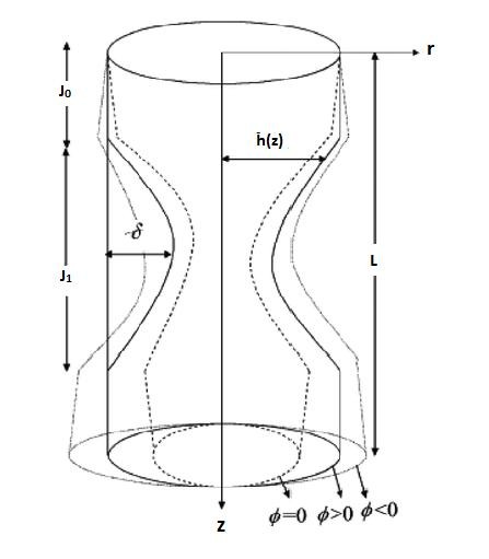
where ϕ is the tapered angle and defined for the non-tapered artery ( ϕ =0), for converging tapering ( ϕ <0), and for diverging tapering ( ϕ >0), as described in Figure  ¹ .

Figure 1

Results and discussion

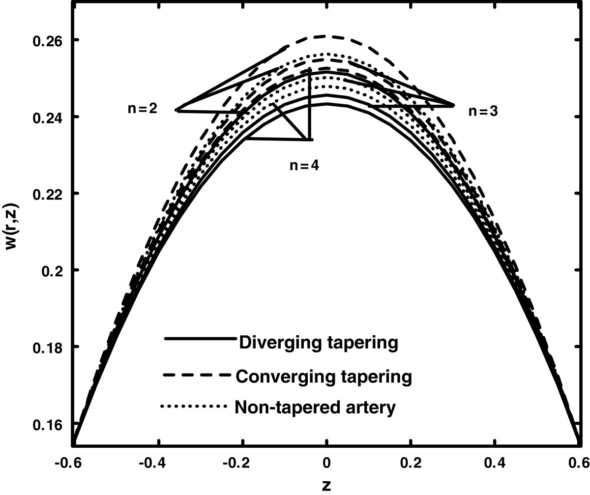
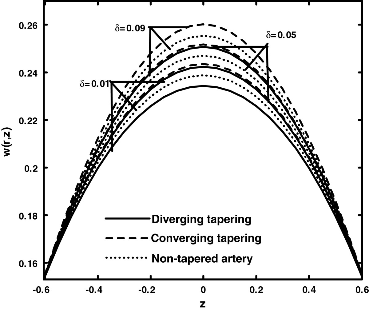
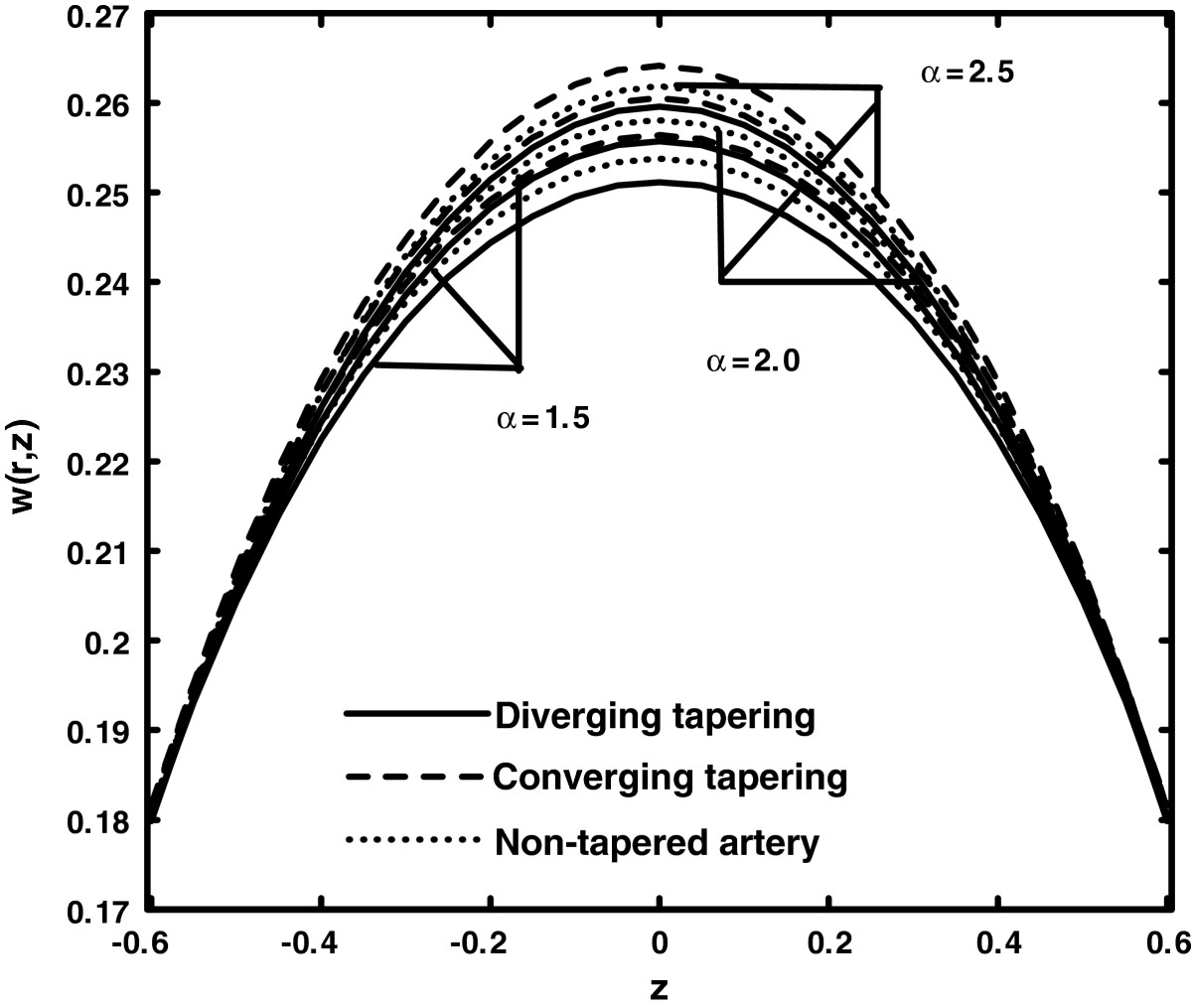
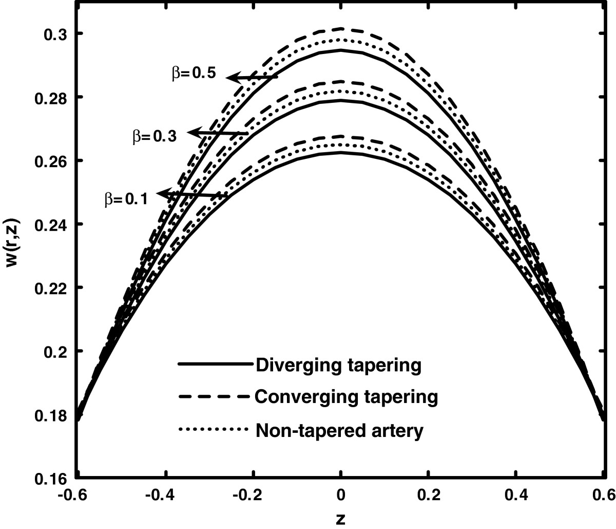
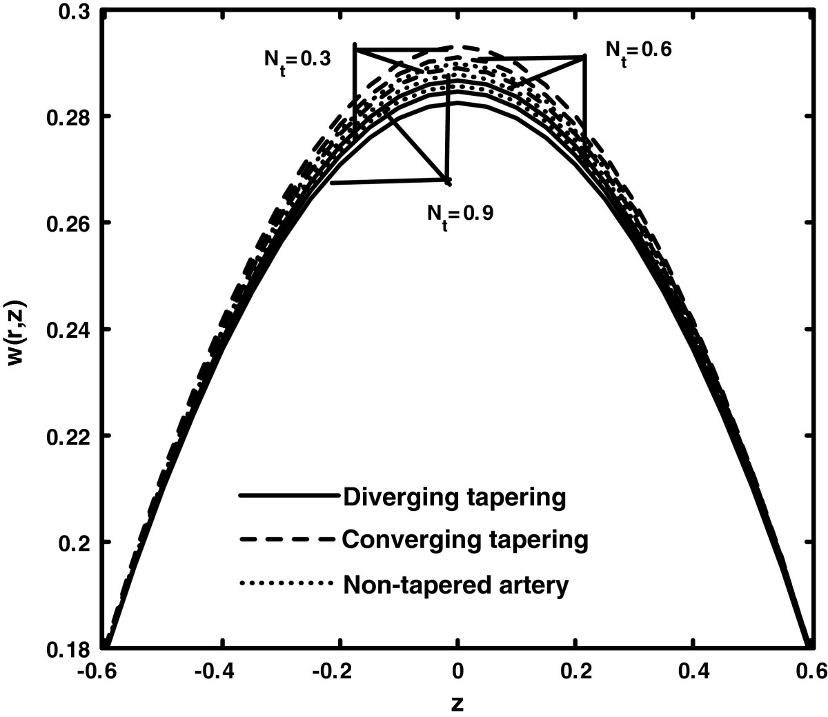
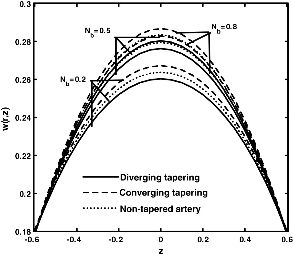
The quantitative results of the α , β , n , δ , N _t , a n d N _b for diverging tapering, converging tapering, and non-tapered arteries are observed physically in Figures ² , ³ , ⁴ , ⁵ , ⁶ , ⁷ , ⁸ , ⁹ , ¹⁰ , ¹¹ , ¹² , ¹³ , ¹⁴ , ¹⁵ , ¹⁶ , ¹⁷ , ¹⁸ , ¹⁹ , ²⁰ , ²¹ , ²² , ²³ , and ²⁴ . Variations of velocity profile for α , β , n , δ , N _t , and N _b for the cases of converging tapering, diverging tapering, and non-tapered arteries are displayed in Figures ² , ³ , ⁴ , ⁵ , ⁶ , and ⁷ . In Figures ² , ³ , ⁴ , ⁵ , ⁶ , and ⁷ , it is analyzed that with an increase in the thermophoresis parameter N _t and stenosis shape n , the velocity profile decreases, while velocity profile increases with an increase in the maximum height of the stenosis δ , Brownian motion parameter N _b , and Prandtl parameters α and β . It is also seen that for the case of converging tapering, it has a larger value as compared with the case of diverging tapering and non-tapered arteries. 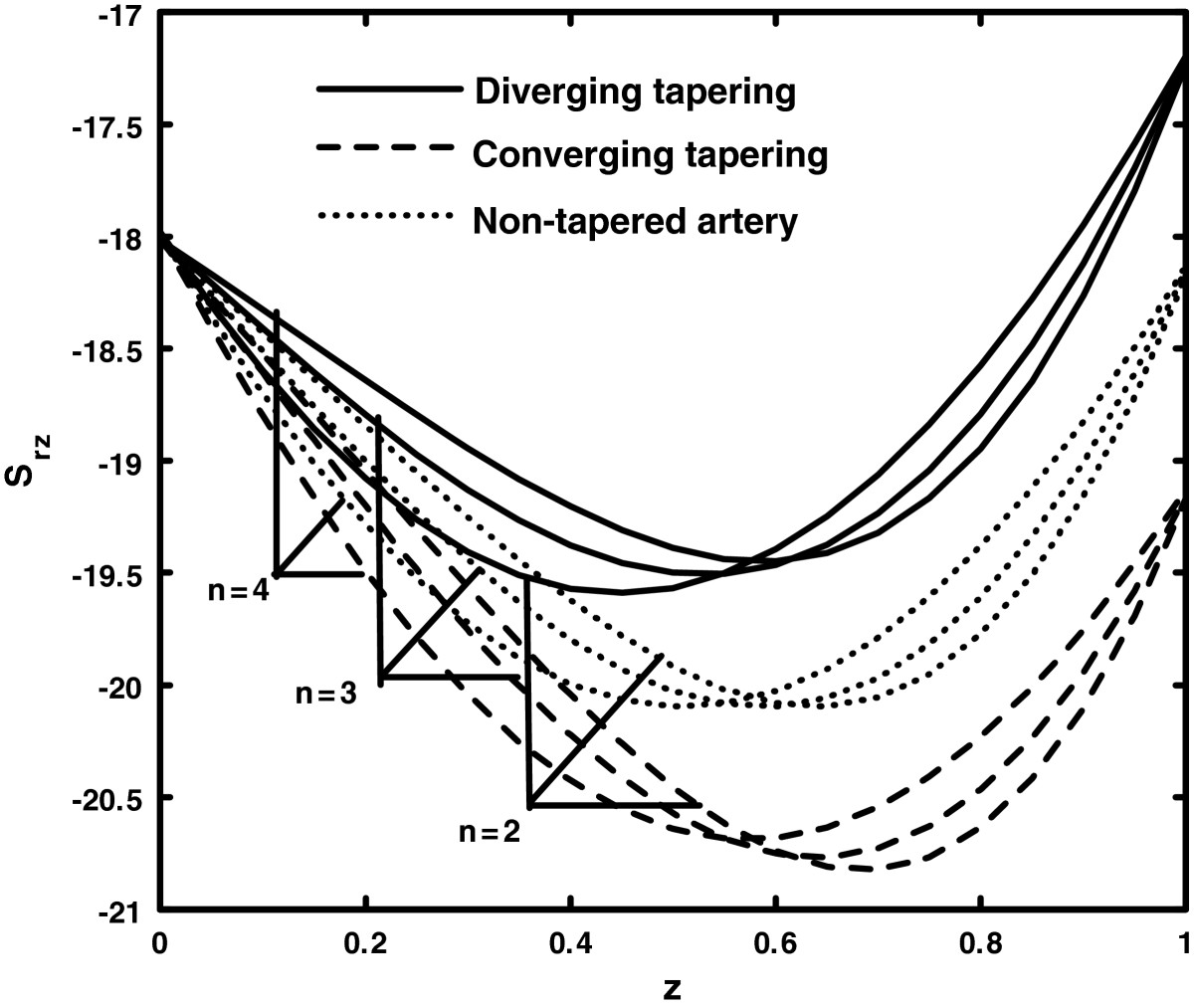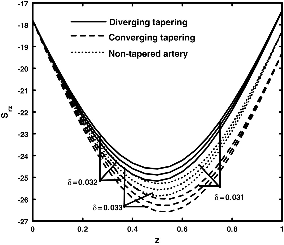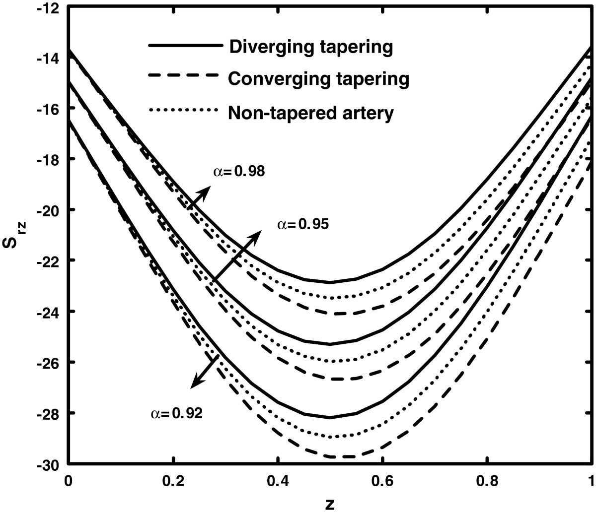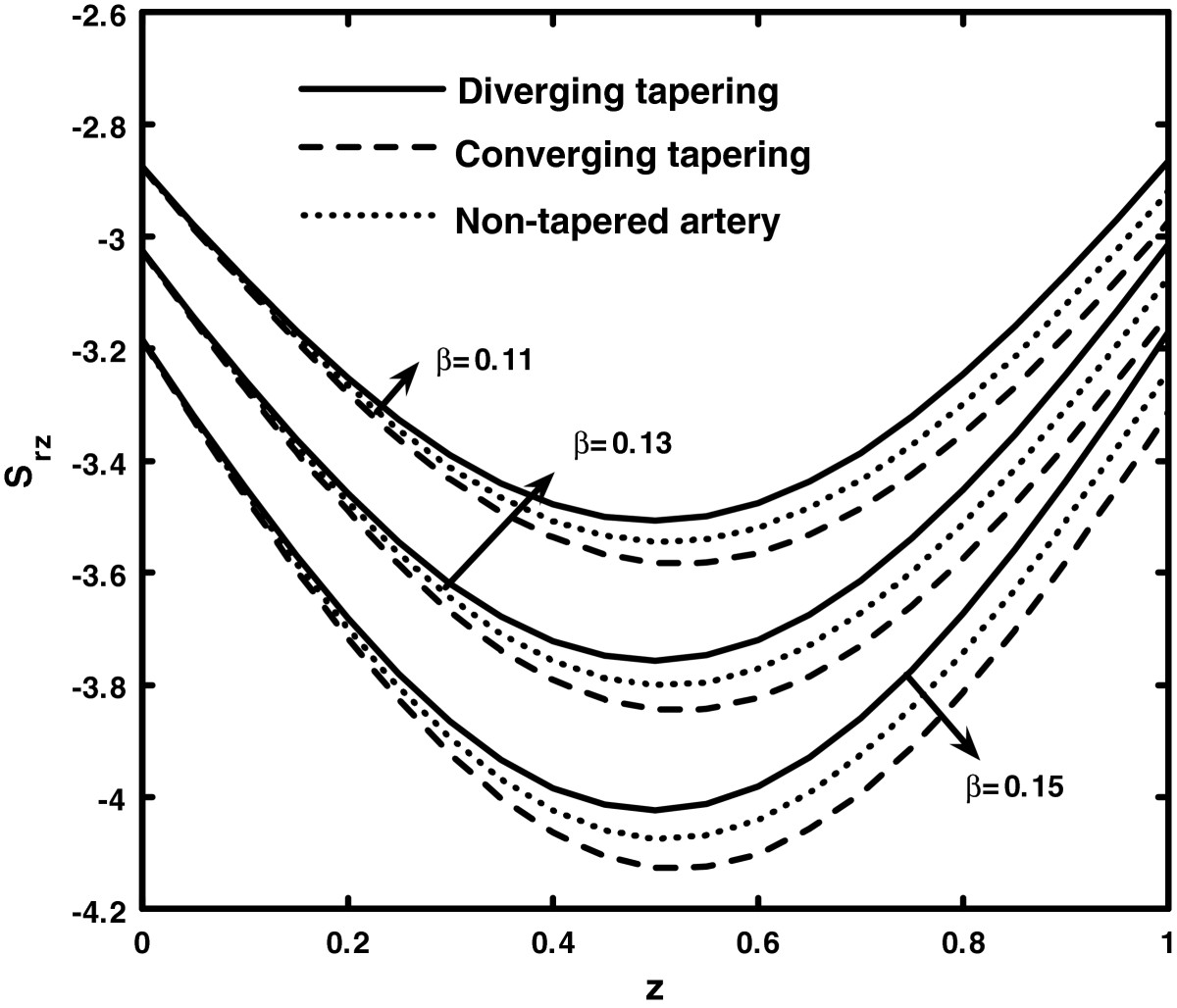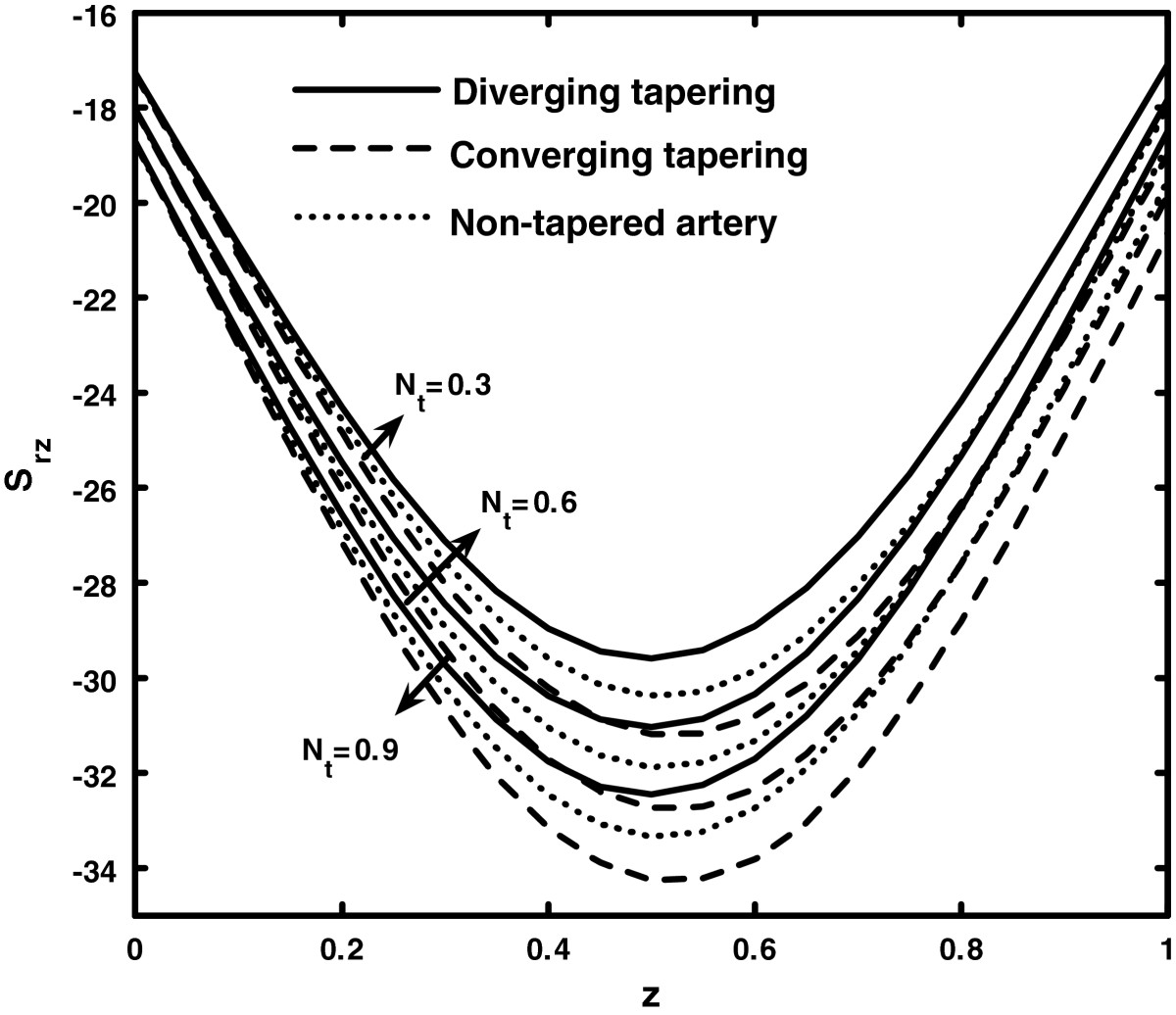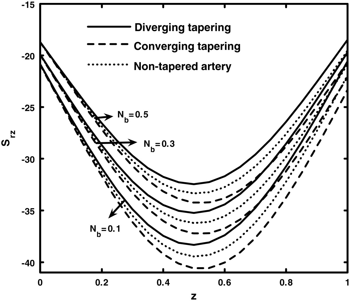Figures ⁸ , ⁹ , ¹⁰ , ¹¹ , ¹² , and ¹³ depict how the converging tapering, diverging tapering, and non-tapered arteries influence the wall shear stress S _{r z} . It is observed that with an increase in stenosis shape n , thermophoresis parameter N _t , stenosis height δ , and Prandtl parameter β , the shear stress decreases, while it increases with an increase in Prandtl parameter α and Brownian motion parameter N _b . 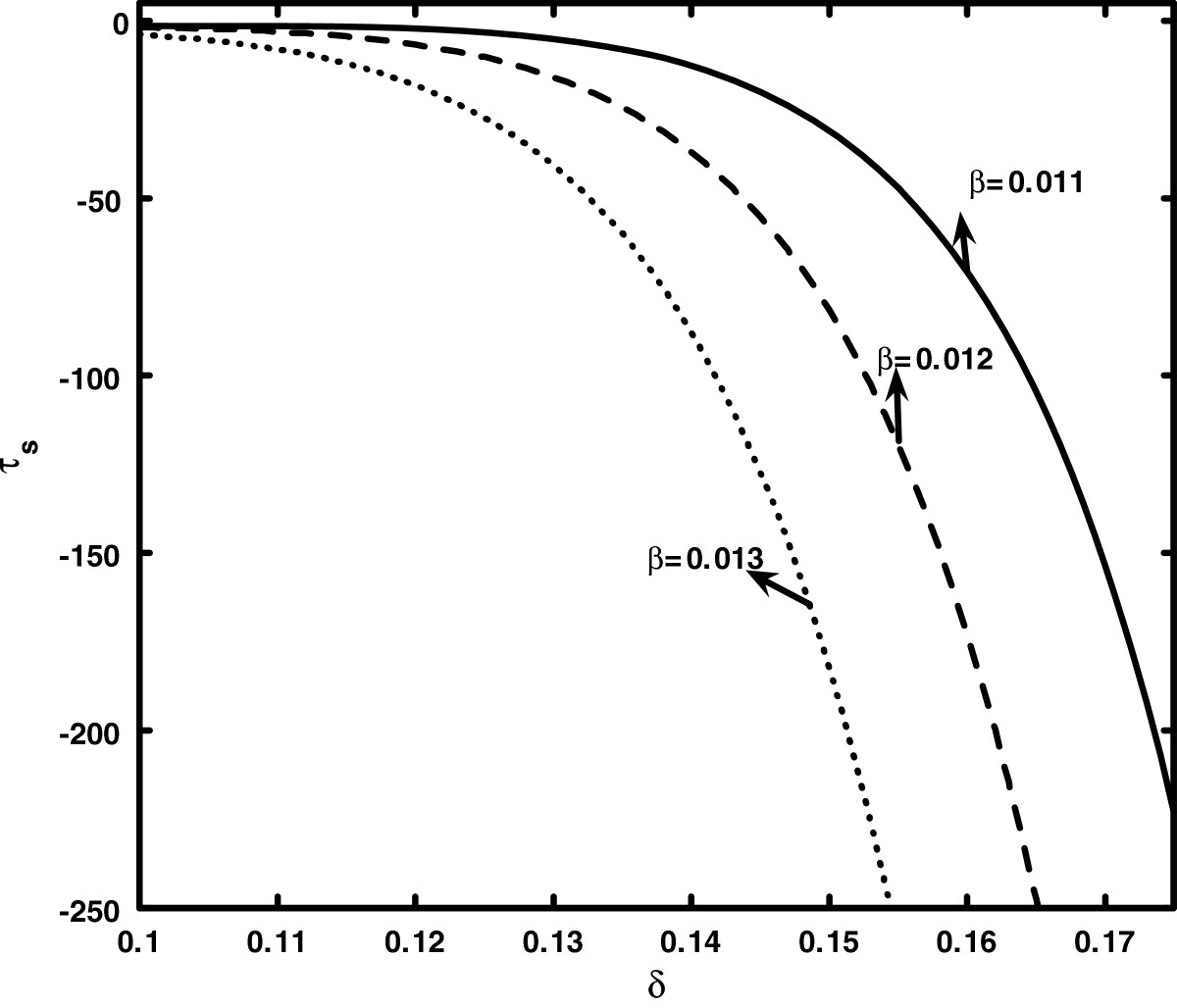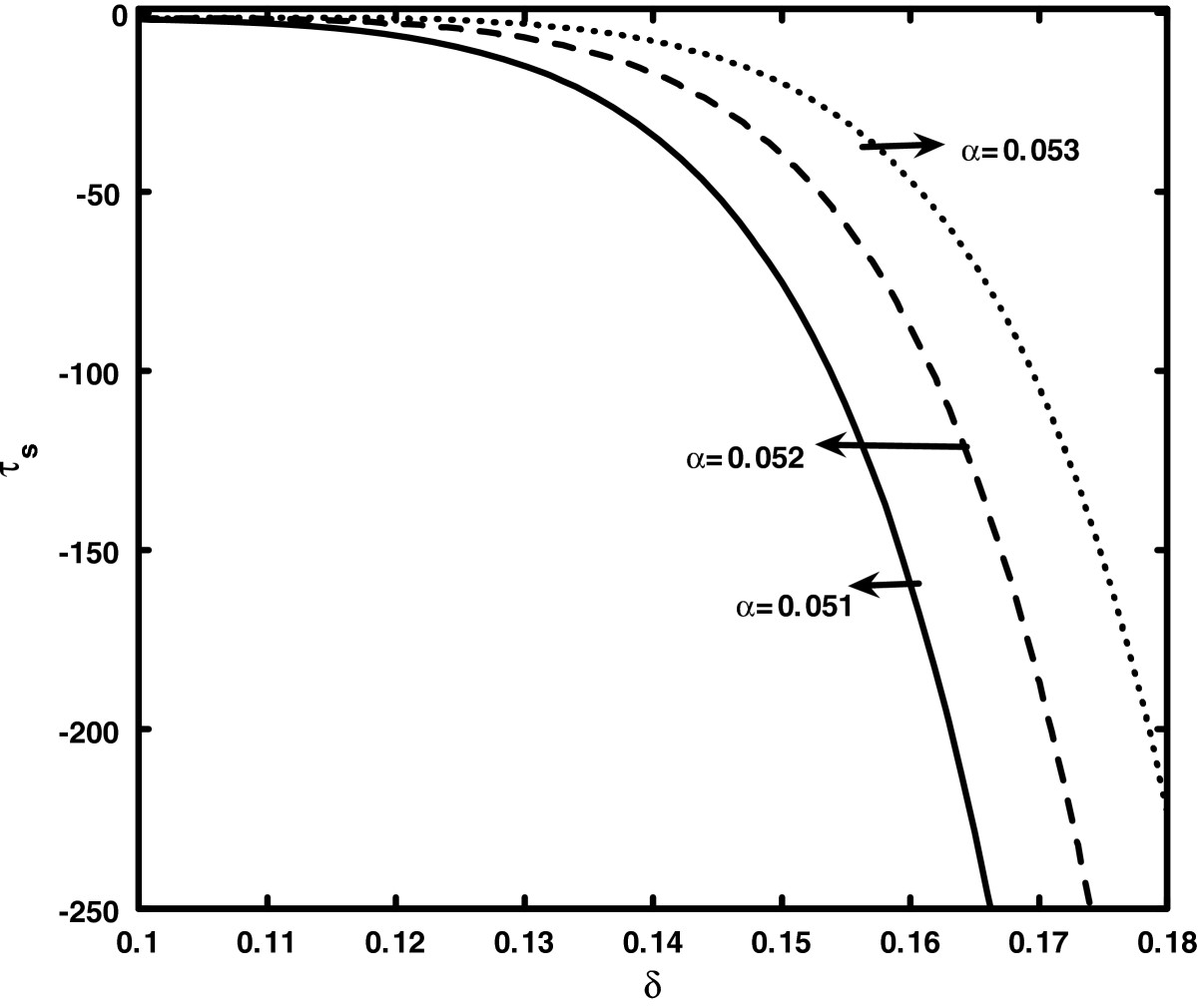Figures ¹⁴ and ¹⁵ depict variations of the shearing stress at the stenosis throat τ _s with δ . In these figures, it is analyzed that the shearing stress at the stenosis throat decreases with an increase in β and increases with an increase in α . 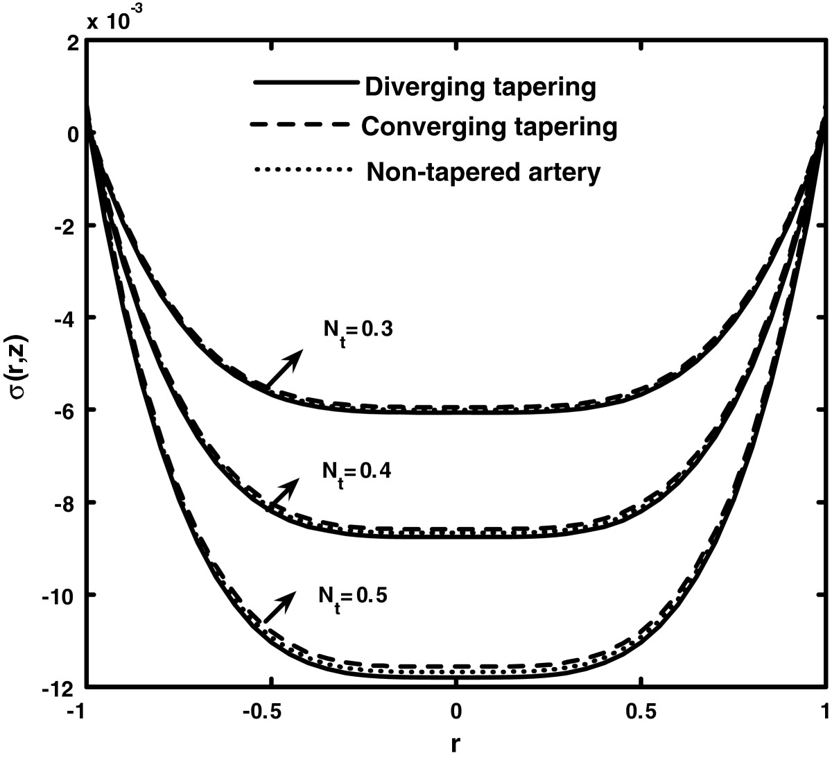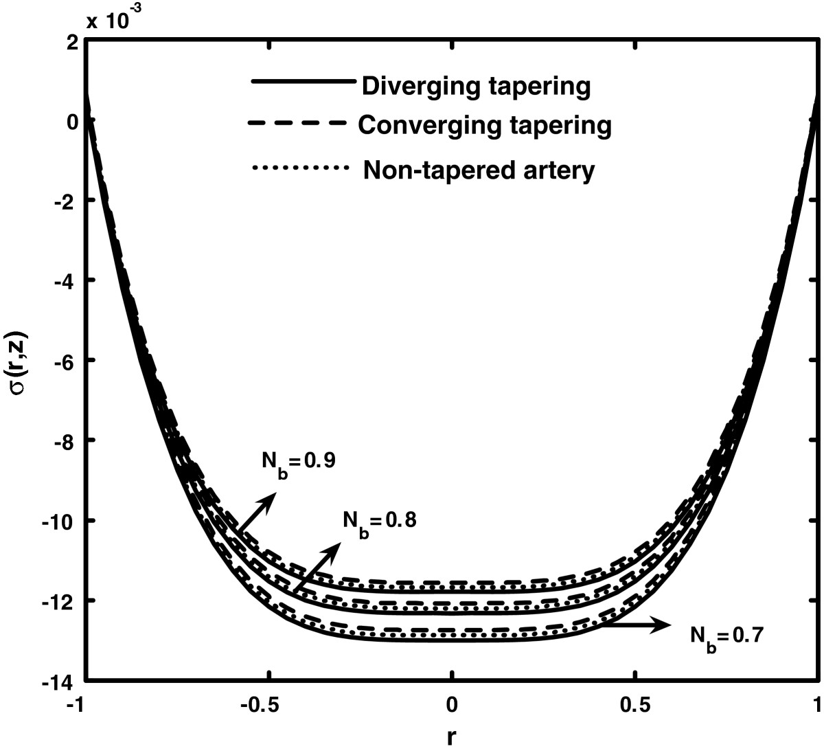Figures ¹⁶ and ¹⁷ show variations of concentration profile for the Brownian motion parameter N _b and thermophoresis parameter N _t . It is observed that with an increase in the Brownian motion parameter N _b , the concentration profile increases, while it decreases with an increase in the thermophoresis parameter N _t and the concentration profile gives a larger value for the converging tapering artery. 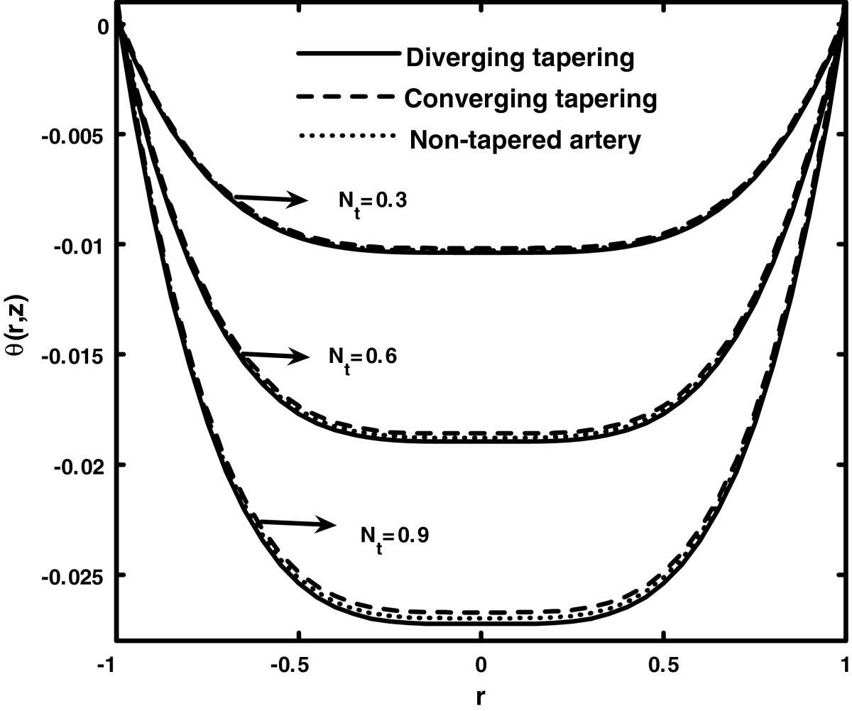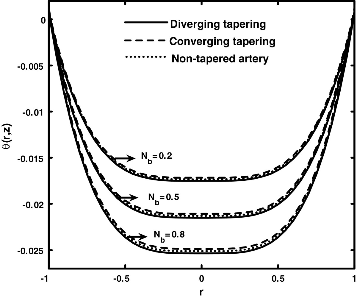Figures ¹⁸ and ¹⁹ depict variations of the temperature profile for the Brownian motion parameter N _b and thermophoresis parameter N _t . It is observed that with an increase in the Brownian motion parameter N _b and the thermophoresis parameter N _t , the temperature profile decreases. 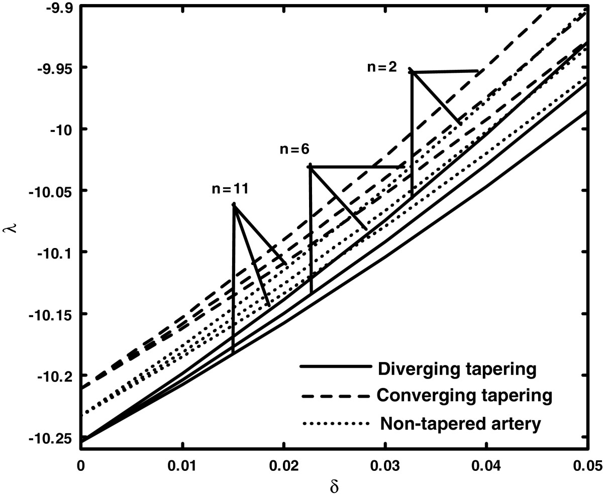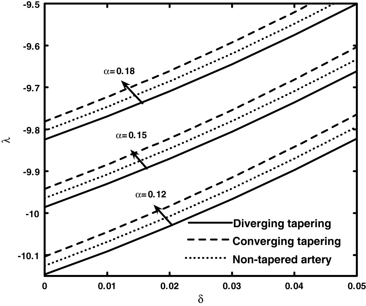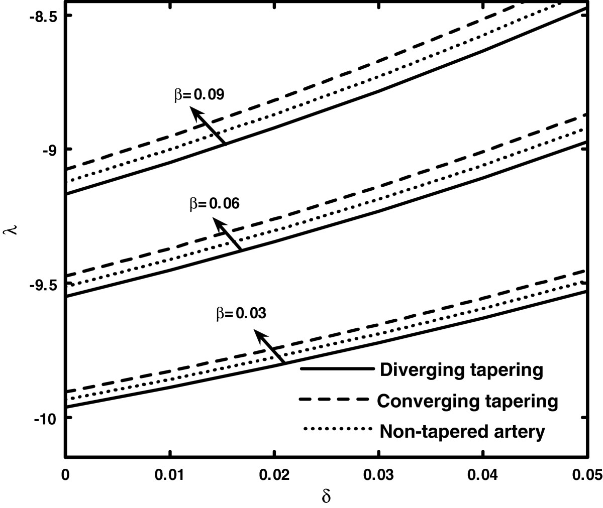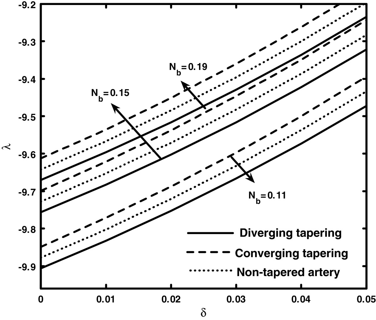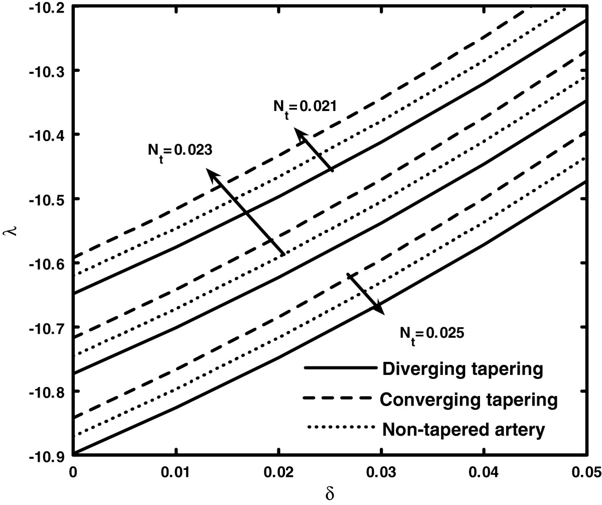Figures ²⁰ , ²¹ , ²² , ²³ , and ²⁴ describe the impedance resistance increases for non-tapered, diverging tapering, and converging tapering arteries when we increase the Prandtl parameters, α , and β , and Brownian motion parameter N _b , while it decreases with an increase in thermophoresis parameters, N _t and n .

Figure 2

Figure 3

Figure 4

Figure 5

Figure 6

Figure 7

Figure 8

Figure 9

Figure 10

Figure 11

Figure 12

Figure 13

Figure 14

Figure 15

Figure 16

Figure 17

Figure 18

Figure 19

Figure 20

Figure 21

Figure 22

Figure 23

Figure 24

Trapping

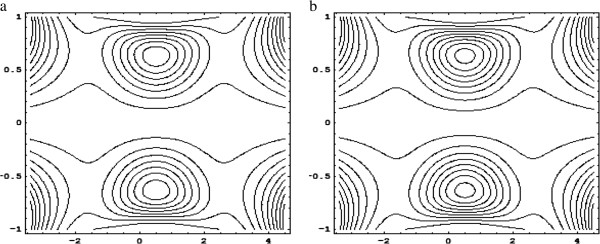
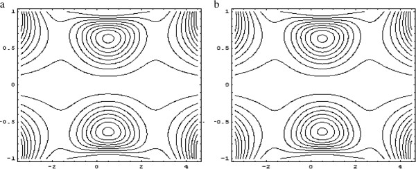
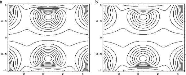
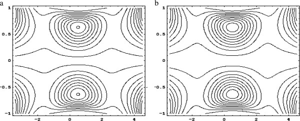
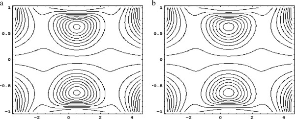
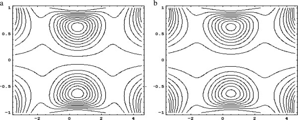
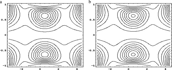
Trapping phenomena can be analyzed in Figures ²⁴ , ²⁵ , ²⁶ , ²⁷ , ²⁸ , ²⁹ , ³⁰ , ³¹ . It is analyzed that with an increase in flow rate F , the number of trapping bolus increases. We also observed that with an increase in β , the size of trapping bolus increases, while the number of trapping bolus increases with an increase in α . It is also observed that with an increase in the Brownian motion parameter N _b , the number of trapping bolus increases, while with an increase in the thermophoresis parameter N _t the number of trapping bolus decreases. It is also analyzed that with local nanoparticle Grashof numbers B _r and G _r , the size of trapping bolus decreases.

Figure 25

Figure 26

Figure 27

Figure 28

Figure 29

Figure 30

Figure 31

Conclusions

The main points of the study that were examined are as follows:

• It is analyzed that with an increase in the thermophoresis parameter N _t and stenosis shape n , the velocity profile decreases, while the velocity profile increases with an increase in the maximum height of the stenosis δ , the Brownian motion parameter N _b , and Prandtl parameters α and β .

• It is analyzed that with an increase in stenosis shape n , the thermophoresis parameter N _t , stenosis height δ , and Prandtl parameter β , the shear stress decreases, while it increases with an increase in the Brownian motion parameter N _b and Prandtl parameter α .

• It is analyzed that the shearing stress at the stenosis throat decreases with an increase in β and increases with an increase in α .

• It is observed that with an increase in the Brownian motion parameter N _b , the concentration profile increases, while it decreases with an increase in the thermophoresis parameter N _t .

• It is observed that with an increase in the Brownian motion parameter, the temperature profile decreases, while with an increase in the thermophoresis parameter, the temperature profile increases.

• It is observed that with an increase in the Brownian motion parameter N _b and the thermophoresis parameter N _t , the temperature profile decreases.

• It is analyzed that with an increase in flow rate F , Prandtl parameter α , and Brownian motion parameter N _b , the number of trapping bolus increases, while it decreases with an increase in the thermophoresis parameter N _t .

• It is also analyzed that the size of trapping bolus decreases with an increase in the local nanoparticle Grashof numbers B _r and G _r , while the size of trapping bolus increases with an increase in the Prandtl parameter β .