In this work, we study the unsteady free convection boundary-layer flow of a nanofluid along a stretching sheet with thermal radiation in the presence of magnetic field. To obtain non-similar equations, continuity, momentum, energy, and concentration equations have been non-dimensionalized by usual transformation. The non-similar solutions are considered here which depend on the magnetic parameter
M
, radiation parameter
R
, Prandtl number
Pr
, Eckert number
Ec
, Lewis number
Le
, Brownian motion parameter
Nb
, thermophoresis parameter
Nt
, and Grashof number
Gr
. The obtained equations have been solved by an explicit finite difference method with stability and convergence analysis. The velocity, temperature, and concentration profiles are discussed for different time steps and for the different values of the parameters of physical and engineering interest.
Background
Magnetohydrodynamics (MHD) boundary-layer flow of nanofluid and heat transfer over a linearly stretched surface have received a lot of attention in the field of several industrial, scientific, and engineering applications in recent years. Nanofluids have many applications in the industries since materials of nanometer size have unique chemical and physical properties. With regard to the sundry applications of nanofluids, the cooling applications of nanofluids include silicon mirror cooling, electronics cooling, vehicle cooling, transformer cooling, etc. This study is more important in industries such as hot rolling, melt spinning, extrusion, glass fiber production, wire drawing, and manufacture of plastic and rubber sheets, polymer sheet and filaments, etc.
Sakiadis [
1
] was the first author to analyze the boundary-layer flow on a continuous surface. Crane [
2
] obtained an exact solution of the boundary-layer flow of the Newtonian fluid caused by the stretching of an elastic sheet moving in its own plane linearly. Gorla et al. [
3
,
4
] solved the non-similar problem of free convective heat transfer from a vertical plate embedded in a saturated porous medium with an arbitrarily varying surface temperature. Cheng and Minkowycz [
5
] also studied free convection from a vertical flat plate with applications to heat transfer from a dick.
Dissipation is the process of converting mechanical energy of downward-flowing water into thermal and acoustical energy. Various devices are designed in streambeds to reduce the kinetic energy of flowing waters, reducing their erosive potential on banks and river bottoms. Vajravelu and Hadjinicalaou [
6
] analyzed the heat transfer characteristics over a stretching surface with viscous dissipation in the presence of internal heat generation or absorption.
Takhar et al. [
7
] studied the radiation effects on the MHD free convection flow of a gas past a semi-infinite vertical plate. Ghaly [
8
] considered the thermal radiation effect on a steady flow, whereas Rapits and Massalas [
9
] and El-Aziz [
10
] analyzed the unsteady case. Sattar and Alam [
11
] presented unsteady free convection and mass transfer flow of a viscous, incompressible, and electrically conducting fluid past a moving infinite vertical porous plate with thermal diffusion effect. Na and Pop [
12
] analyzed an unsteady flow due to a stretching sheet. In the case of unsteady boundary-layer flow, Singh et al. [
13
] investigated the thermal radiation and magnetic field effects on an unsteady stretching permeable sheet in the presence of free stream velocity. The study of convective instability and heat transfer characteristics of nanofluids was considered by Kim et al. [
14
]. Jang and Choi [
15
] obtained nanofluid thermal conductivity and the effect of various parameters on it.
The natural convective boundary-layer flows of a nanofluid past a vertical plate have been described by Kuznetsov and Nield [
16
,
17
]. In this model, the Brownian motion and thermophoresis are accounted with the simplest possible boundary conditions. They also studied the Cheng-Minkowycz problem for natural convective boundary-layer flow in a porous medium saturated by a nanofluid. Bachok et al. [
18
] have shown the steady boundary-layer flow of a nanofluid past a moving semi-infinite flat plate in a uniform free stream. It was assumed that the plate is moving in the same or opposite directions to the free stream to define the resulting system of non-linear ordinary differential equations.
Khan and Pop [
19
,
20
] formulated the problem of laminar boundary-layer flow of a nanofluid past a stretching sheet. They also expressed free convection boundary-layer nanofluid flow past a horizontal flat plate. Hamad and Pop [
21
] discussed the boundary-layer flow near the stagnation-point flow on a permeable stretching sheet in a porous medium saturated with a nanofluid. Hamad et al. [
22
] investigated free convection flow of a nanofluid past a semi-infinite vertical flat plate with the influence of magnetic field. Very recently, Hady et al. [
23
] investigated the effects of thermal radiation on the viscous flow of a nanofluid and heat transfer over a non-linearly stretching sheet.
However, the aim of the present work is to study the unsteady free convection boundary-layer nanofluid flows along a stretching surface with the influence of magnetic field and radiation effect. An explicit finite difference procedure [
24
] has been taken to solve the obtained non-similar equations with stability and convergence analysis.
Methods
Presentation of the hypothesis
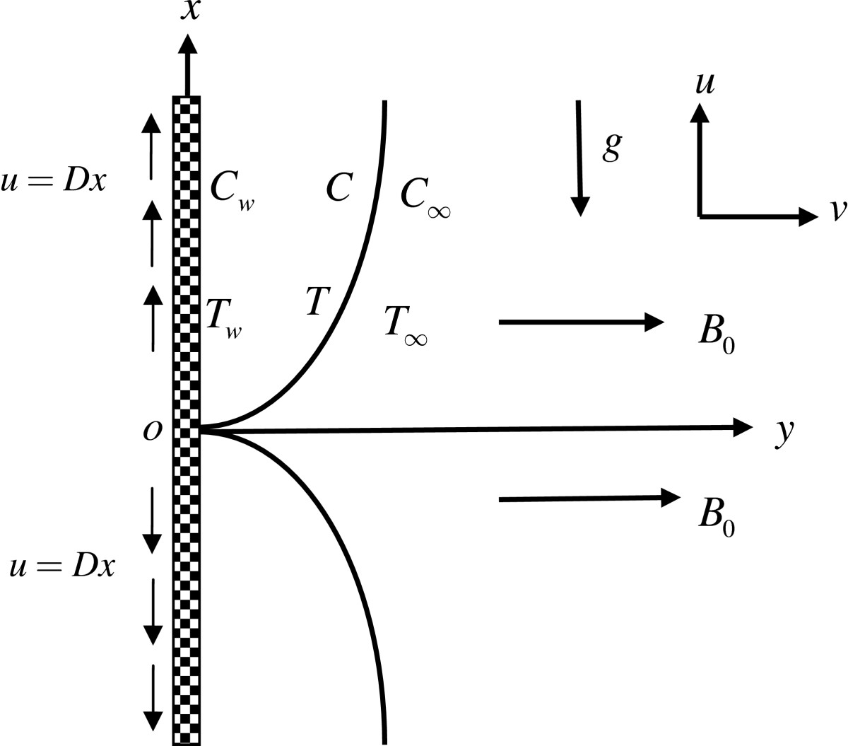
An unsteady two-dimensional MHD free convection laminar boundary-layer flow of a viscous incompressible and electrically conducting nanofluid along a vertical stretching sheet under the influence of thermal radiation and viscous dissipation is considered. The sketch of the physical configuration and coordinate system is shown in Figure
1
. Introducing the Cartesian coordinate system, the
x
-axis is taken along the stretching sheet in the vertically upward direction, and the
y
-axis is taken as normal to the sheet. Two equal and opposite forces are introduced along the
x
-axis so that the sheet is stretched, keeping the origin fixed.
Figure 1
Physical model and coordinate system.
Instantaneously at time
t
> 0, the temperature of the plate and the species concentration are raised to
Tw
(>
T∞
) and
Cw
(>
C∞
), respectively, which are thereafter maintained constant, where
Tw
and
Cw
are the temperature and species concentration at the wall, respectively, and
T∞
and
C∞
are the temperature and species concentration far away from the plate, respectively.
A strong magnetic field is applied in the
y
direction. The uniform magnetic field strength (magnetic induction)
B0
can be taken as
B
= (0,
B0
, 0). The Rosseland approximation is used to describe the radioactive heat flux
qr
in the energy equation. Under the above assumptions and the usual boundary layer approximation, the MHD free convection unsteady nanofluid flow and heat and mass transfer with the radiation effect are governed by the following equations:
The continuity equation
∂u∂x+∂v∂y=0
The momentum equation
∂u∂t+u∂u∂x+v∂u∂y=υ∂2u∂y2+gβT-T∞-σB02uρ
The energy equation
∂T∂t+u∂T∂x+v∂T∂y=kρcp∂2T∂y2-1ρcp∂qr∂y+υcp∂u∂y2+τDB∂T∂y·∂C∂y+DTT∞∂T∂y2
The concentration equation
∂C∂t+u∂C∂x+v∂C∂y=DB∂2C∂y2+DTT∞∂2T∂y2
The initial and boundary conditions are
t=0,u=Dx,v=0,T=T∞,C=C∞everywheret≥0,u=0,v=0,T=T∞,C=C∞atx=0u=Dx,v=0,T=Tw,C=Cwaty=0u=0,v=0,T→T∞,C→C∞aty→∞,
where
u
and
v
are the velocity components in the
x
and
y
directions, respectively,
v
is the kinematic viscosity,
k
is the thermal conductivity,
DB
is the Brownian diffusion coefficient,
DT
is the thermophoresis diffusion coefficient,
D
(> 0) is the stretching constant,
g
is the acceleration due to gravity,
ρ
is the density of the fluid, and
cp
is the specific heat at constant pressure.
The Rosseland approximation [
25
] is expressed for radiative heat flux and leads to the form
qr=-4σ3κ*∂T4∂y,
where
σ
is the Stefan-Boltzmann constant and
κ*
is the mean absorption coefficient. The temperature difference within the flow is sufficiently small such that
T4
may be expressed as a linear function of the temperature, then Taylor's series for
T4
is about
T∞
after neglecting higher order terms:
T4=4T∞3-3T∞4.
Introducing the following non-dimensional variables,
X=xU0υ,Y=yU0υ,U=uU0,V=vU0,τ=tU02υ,T―=T-T∞Tw-T∞,C―=C-C∞Cw-C∞.
Then, Equations
1
to
5
become
∂U∂X+∂V∂Y=0∂U∂τ+U∂U∂X+V∂U∂Y=∂2U∂Y2+GrT―-MU∂T―∂τ+U∂T―∂X+V∂T―∂Y=1+RPr·∂2T―∂Y2+Ec∂U∂Y2+Nb∂T―∂Y·∂C―∂Y+Nt∂T―∂Y2∂C―∂τ+U∂C―∂X+V∂C―∂Y=1Le∂2C―∂Y2+NtNb∂2T―∂Y2.
The non-dimensional boundary conditions are
τ≤0,U=0,V=0,T―=0,C―=0everywhereτ>0,U=0,V=0,T―=0,C―=0atX=0U=1,V=0,T―=1,C―=1atY=0U=0,V=0,T―=0,C―=0asY→∞,
where the magnetic parameter
M=σB02νρU02
, Grashof number
Gr=gβTw-T∞νUo3
, radiation parameter
R=16σT∞33kκ*
, Prandtl number
Pr=υα
, Eckert number
Ec=U02cpTw-T∞
, Lewis number
Le=υDB
, Brownian parameter
Nb=τDBCw-C∞υ
, and thermophoresis parameter
Nt=DTT∞τνTw-T∞
.
Methods: numerical computation
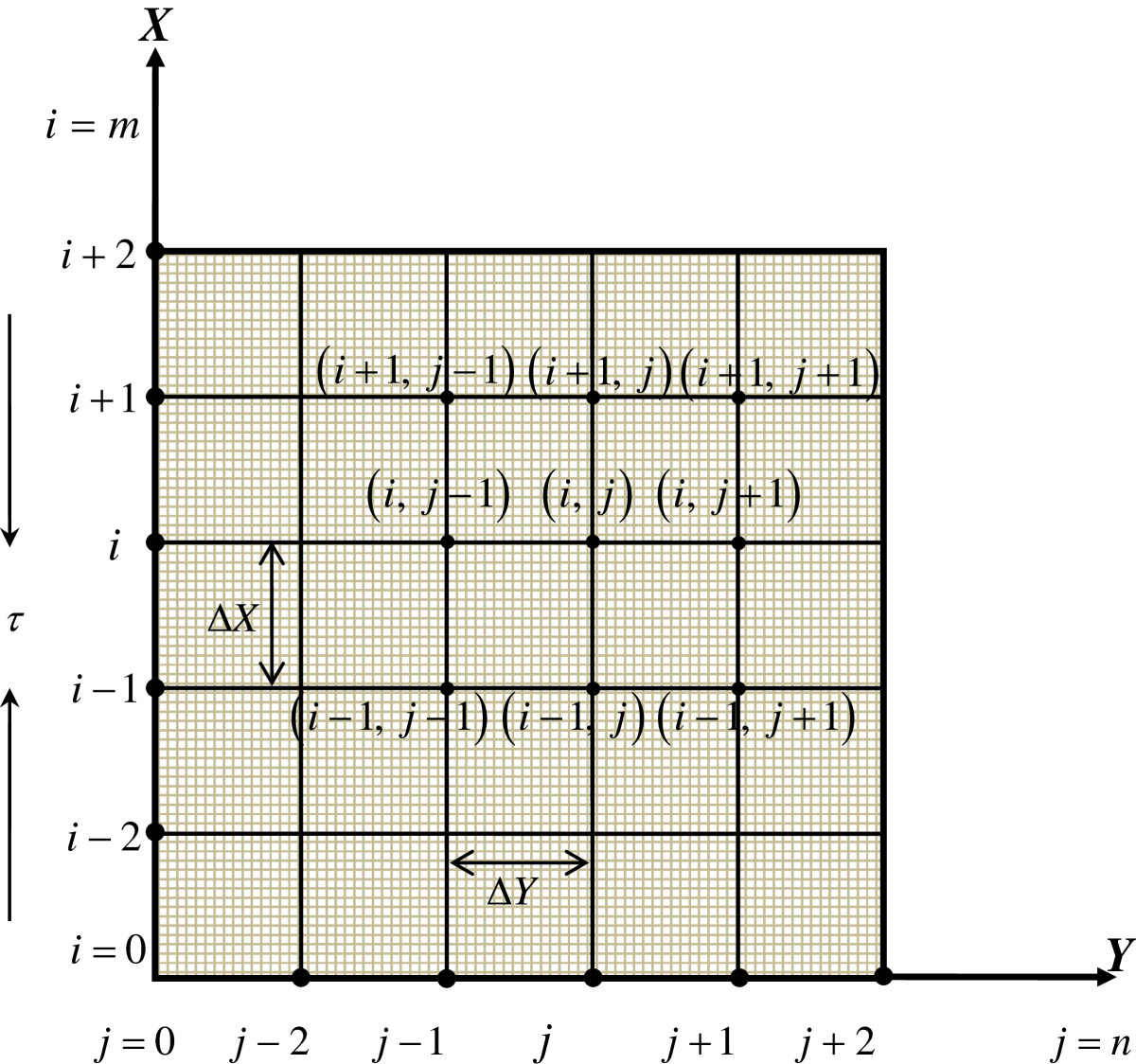
In order to solve the non-similar unsteady coupled non-linear partial differential equations (Equations 8, 9, 10, and 11), the explicit finite difference method has been developed. For this, a rectangular region of the flow field is chosen, and the region is divided into a grid of lines parallel to
X
and
Y
axes, where the
X
-axis is taken along the plate and the
Y
-axis is normal to the plate.
Here, the plate of height
Xmax
(=100) is considered, i.e.,
X
varies from 0 to 100 and assumed
Ymax
(=25) as corresponding to
Y
→
∞
, i.e.,
Y
varies from 0 to 25. There are
m
(=125) and
n
(=125) grid spacing in the
X
and
Y
directions, respectively, as shown in Figure
2
. It is assumed that
ΔX
and
ΔY
are constant mesh sizes along the
X
and
Y
directions, respectively, and taken as follows: Δ
X
= 0.8(0 ≤
X
≤ 100) and Δ
Y
= 0.2(0 ≤
Y
≤ 25) with the smaller timestep Δ
τ
= 0.005.
Figure 2
Finite difference space grid.
Let
U′
,
V′
,
T―′
, and
C―′
denote the values of
U
,
V
,
T―
, and
T―
at the end of a time step, respectively. Using the explicit finite difference approximation, the following appropriate sets of finite difference equations are obtained:
U′i,j-U′i-1,jΔX+Vi,j-Vi,j-1ΔY=0U′i,j-Ui,jΔτ+Ui,jUi,j-Ui-1,jΔX+Vi,jUi,j+1-Ui,jΔY=Ui,j+1-2Ui,j+Ui,j-1ΔY2+GrT′-MUi,jT―′i,j-T―i,jΔτ+Ui,jT―i,j-T―i-1,jΔX+Vi,jT―i,j+1-T―i,jΔY=1+RPrT―i,j+1-2T―i,j+T―i,j-1ΔY2+EcUi,j+1-Ui,jΔY2+NbT―i,j+1-T―i,jΔY·C―i,j+1-C―i,jΔY+NtT―i,j+1-T―i,jΔY2C′―i,j-C―i,jΔτ+Ui,jC―i,j-C―i-1,jΔX+Vi,jC―i,j+1-C―i,jΔY=1LeC―i,j+1-2C―i,j+C―i,j-1ΔY2+NtNbT―i,j+1-2T―i,j+T―i,j-1ΔY2
with initial and boundary conditions
Ui,j0=0,Vi,j0=0,T―i,j0=0,C―i,j0=0U0,jn=0,V0,jn=0,T―0,j0=0,C―0,jn=0Ui,0n=1,Vi,0n=0,T―i,0n=1,C―i,0n=1Ui,Ln=0,Vi,Ln=0,T―i,Ln=0,C―i,Ln=0,whereL→∞,
where the subscripts
i
and
j
designate the grid points with
X
and
Y
coordinates, respectively, and the superscript
n
represents a value of time,
τ
=
n
·
Δτ
, where
n
= 0, 1, 2, ….
Stability and convergence analysis
Since an explicit procedure is being used, the analysis will remain incomplete unless the stability and convergence of the finite difference scheme is discussed. For the constant mesh sizes, the stability criteria of the scheme may be established as follows.
Equation 14 will be ignored since
Δτ
does not appear in it. The general terms of the Fourier expansion for
U
,
T―
, and
C―
at a time arbitrarily called
τ
= 0 are all
eiαXeiβY
, apart from a constant, where
i=-1
. At a time
τ
, these terms become
U:ψτeiαXeiβYT―:θτeiαXeiβYC―:ϕτeiαXeiβY,
and after the time step, these terms will become
U:ψ′τeiαXeiβYT―:θ′τeiαXeiβYC―:ϕ′τeiαXeiβY.
Substituting Equations
20
and
21
into Equations
15
to
17
, with regard to the coefficients
U
and
V
as constants over any one time step, we obtain the following equations upon simplification:
ψ′τ-ψτΔτ+Uψτ1-e-iαΔXΔX+VψτeiβΔY-1ΔY=2ψτcosβΔY-1ΔY2+Grθ′τ-Mψτθ′τ-θτΔτ+Uθτ1-e-iαΔXΔX+VθτeiβΔY-1ΔY=1+RPr2θτcosβΔY-1ΔY2+EcUψτeiβΔY-1ΔY2+NbC―θτeiβΔY-1ΔY2+NtT―θτeiβΔY-1ΔY2ϕ′τ-ϕτΔτ+Uϕτ1-e-iαΔXΔX+VϕτeiβΔY-1ΔY=1Le2ϕτcosβΔY-1ΔY2+NtNb·2θτcosβΔY-1ΔY2
Equations 22, 23, and 24 can be written in the following forms:
ψ′=Aψ+GrΔτθ/θ′=Bθ+Eψϕ′=Jϕ+Kθ,
where
A=1-UΔτΔX1-e-iαΔX-VΔτΔYeiβΔY-1+2ΔτΔY2cosβΔY-1-MΔτB=1-UΔτΔX1-e-iαΔX-VΔτΔYeiβΔY-1+1+RPr2cosβΔY-1ΔY2Δτ+NbC―eiβΔY-1ΔY2Δτ+NtT―eiβΔY-1ΔY2Δτ,E=EcUΔτΔY2eiβΔY-12,J=1-UΔτΔX1-e-iαΔX-VΔτΔYeiβΔY-1+1Le2ΔτΔY2cosβΔY-1,
and
K=1LeNtNb2ΔτΔY2cosβΔY-1.
Again using Equation
26
in Equation
25
,
ψ′=Aψ+GrΔτBθ+Eψ=Cψ+Dθ,
where
C
=
A
+
EGr
Δ
τ
and
D
=
BGr
Δ
τ
.
Therefore, Equations
25
,
26
, and 27 can be expressed as
ψ′=Cψ+Dθθ′=Bθ+Eψϕ′=Jϕ+Kθ.
Hence, Equations
28
,
29
, and 30 can be expressed in a matrix notation, and these equations are
ψ′θ′ϕ′=CD00B00KJ.ψθϕ,
that is,
η′
=
Tη
, where
η′=ψ′θ′ϕ′,T=CD00B00KJ.andη=ψθϕ.
For obtaining the stability condition, we have to find out eigenvalues of the amplification matrix
T
, but this study is very difficult since all the elements of
T
are different. Hence, the problem requires that the Eckert number
Ec
is assumed to be very small, that is, tends to zero. Under this consideration, we have
E
= 0, and the amplification matrix becomes
T=CD00B00KJ.
After simplification of the matrix
T
, we get the following eigenvalues:
λ1
=
C
,
λ2
=
B
, and
λ3
=
J
.For stability, each eigenvalue (
λ1
,
λ2
, and
λ3
) must not exceed unity in modulus. Hence, the stability condition is|
C
| ≤ 1, |
B
| ≤ 1, and
J
≤ 1, for all
a
,
β
.
Now, we assume that
U
is everywhere non-negative and
V
is everywhere non-positive. Thus,
B=1-2a+b+2c1+RPr+NbC―+NtT―,
where
a=UΔτΔX,b=VΔτΔYandc=ΔτΔY2.
The coefficients
a
,
b
, and
c
are all real and non-negative. We can demonstrate that the maximum modulus of
B
occurs when
α
Δ
X
=
mπ
and
β
Δ
Y
=
nπ
, where
m
and
n
are integers; hence,
B
is real. The value of |
B
| is greater when both
m
and
n
are odd integers.
To satisfy the second condition |
B
| ≤ 1, the most negative allowable value is
B
= - 1. Therefore, the first stability condition is
2a+b+2c1+RPr+NbC―+NtT―≤2,
that is,
UΔτΔX+VΔτΔY+21+RPrΔτΔY2+2NbC―ΔτΔY2+2NtT―ΔτΔY2≤1.
Likewise, the third condition |
J
| ≤ 1 requires that
UΔτΔX+VΔτΔY+2LeΔτΔY2≤1.
Therefore, the stability conditions of the method are
UΔτΔX+VΔτΔY+21+RPrΔτΔY2+2NbC―ΔτΔY2+2NtT―ΔτΔY2≤1andUΔτΔX+VΔτΔY+2LeΔτΔY2≤1.
Since, from the initial condition,
U=V=T―=C―=0
at
τ
= 0, the consideration due to stability and convergence analysis is
Ec
< < 1 and
R
≥ 0.5. Hence, convergence criteria of the method are
Pr
≥ 0.37 and
Le
≥ 0.25.
Results and discussion
In order to investigate the problem under consideration, the results of numerical values of non-dimensional velocity, temperature, and species concentration within the boundary layer have been computed for different values of magnetic parameter
M
, radiation parameter
R
, Prandtl number
Pr
, Eckert number
Ec
, Lewis number
Le
, Brownian motion parameter
Nb
, thermophoresis parameter
Nt
, and Grashof number
Gr
, respectively. To obtain the steady-state solutions of the computation, the calculations have been carried out up to non-dimensional time
τ
= 5 to 80. The velocity, temperature, and concentration profiles do not show any change after non-dimensional time
τ
= 50. Therefore, the solution for
τ
≥ 50 is the steady-state solution. The graphical representation of the problem has been shown in Figures
3
,
4
,
5
,
6
,
7
,
8
,
9
, and
10
.
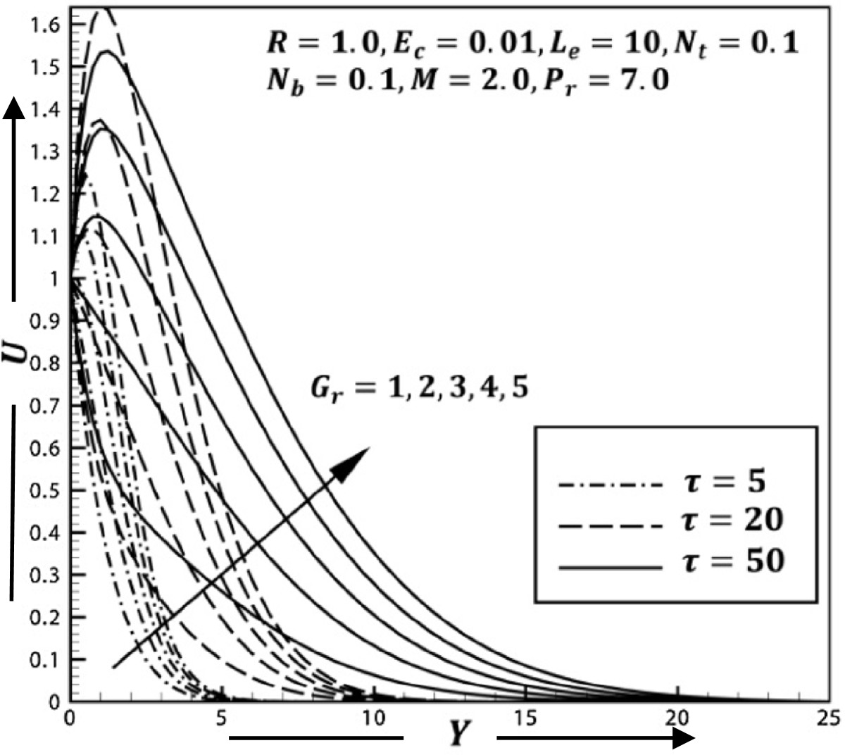
Figure 3
Grashof number (Gr) effect on velocity profiles.
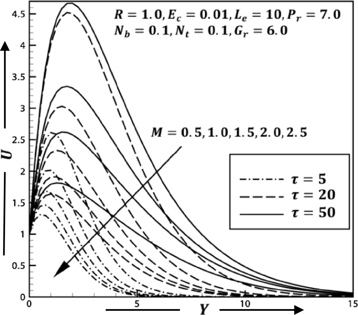
Figure 4
Magnetic parameter (M) effect on velocity profiles.
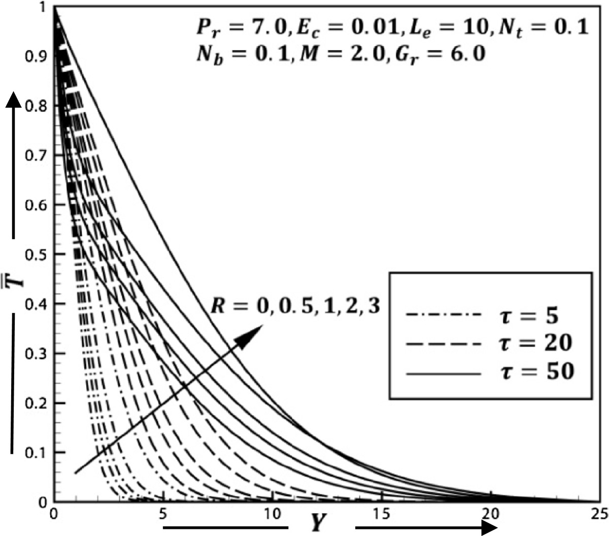
Figure 5
Radiation parameter (R) effect on temperature profiles.
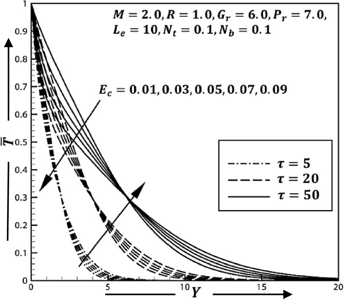
Figure 6
Eckert number (Ec) effect on temperature profiles.
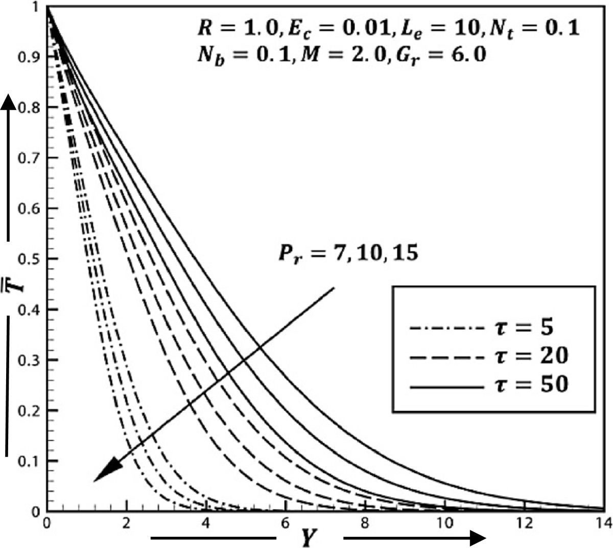
Figure 7
Prandtl number (Pr) effect on temperature profiles.
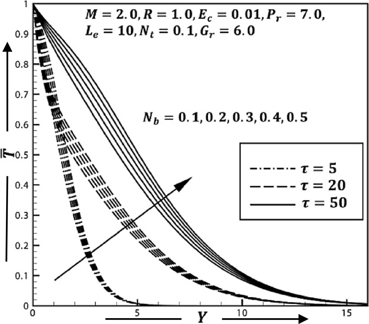
Figure 8
Brownian parameter (Nb) effect on temperature profiles.
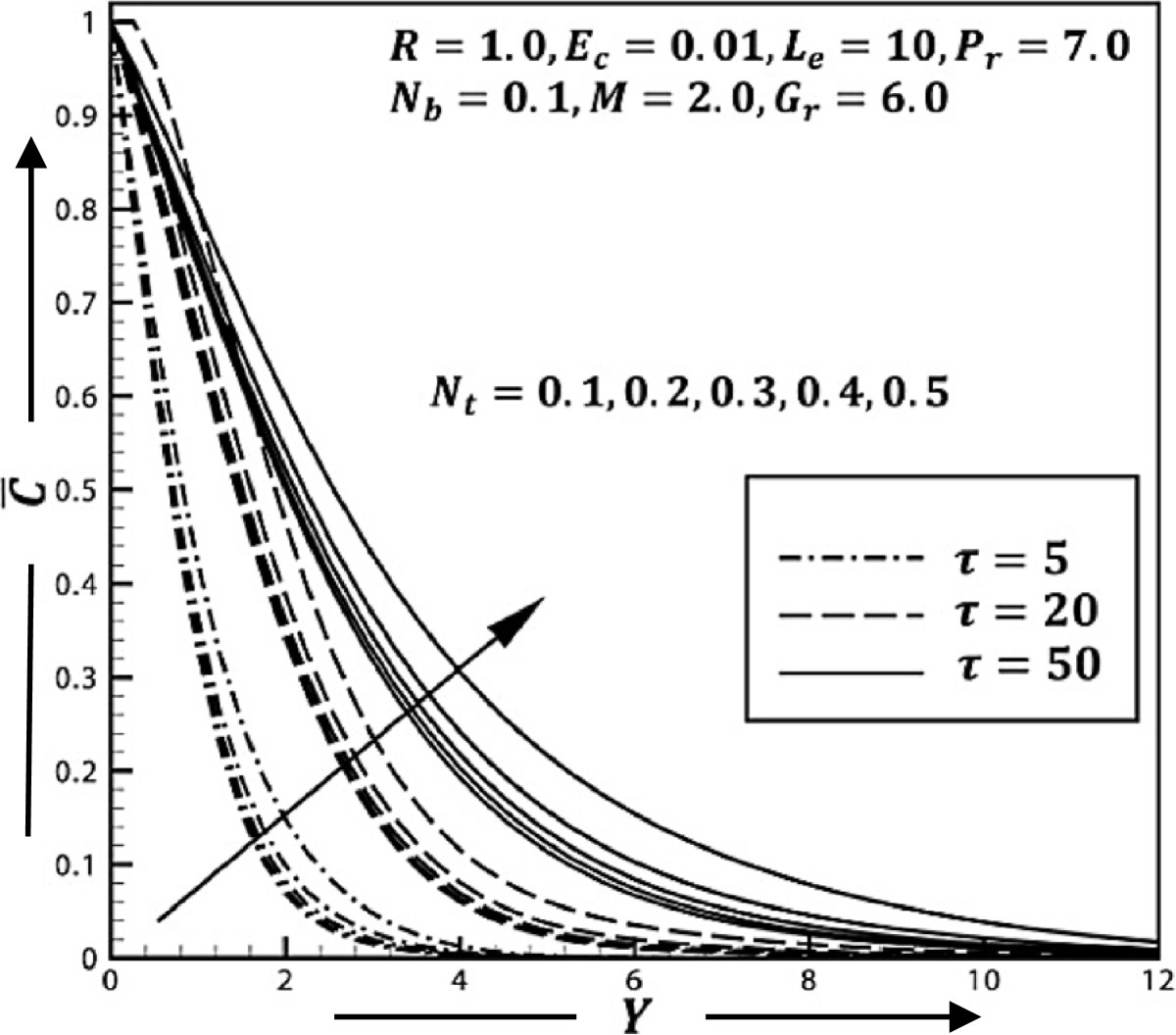
Figure 9
Thermophoresis parameter (Nt) effect on concentration profiles.
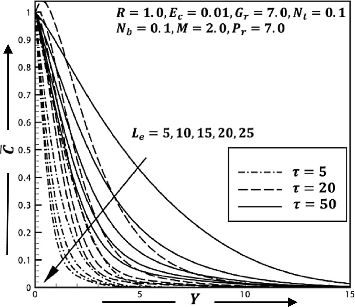
Figure 10
Lewis number (Le) effect on concentration profiles.
In order to assess the accuracy of the numerical results, the present results (non-similar solution) are compared with the result obtained by Khan and Pop [
19
] (similar solution) and the values of magnetic parameter
M
, radiation parameter
R
, Eckert number
Ec
, and Grashof number
Gr
are considered zero (Table
1
). From the comparison, excellent agreement is observed.
Table 1
Comparison of results for the reduced Nusselt numberNu=-1ΔT∂T∂yy=0whenM = Gr = R = Ec = 0 andPr = Le = 10
Non-dimensional time
Parameter
Present results
Khan and Pop's [[19]] results
(τ)
Nt = Nb =
(non-similar solution)
(similar solution)
60
0.1
0.9541
0.9524
60
0.2
0.3667
0.3654
60
0.3
0.1359
0.1355
60
0.4
0.0499
0.0495
60
0.5
0.0185
0.0179
In Figures
3
,
4
,
5
,
6
,
7
,
8
,
9
, and
10
, the dimensionless velocity, temperature, and concentration distributions are plotted against
Y
for the different non-dimensional time
τ
= 5 to 50 and corresponding values of Grashof number
Gr
, magnetic parameter
M
, radiation parameter
R
, Eckert number
Ec
, Prandtl number
Pr
, Brownian motion parameter
Nb
, thermophoresis parameter
Nt
, and Lewis number
Le
, respectively.
In Figures
3
and
4
, the velocity distribution is plotted respectively for different values of
Gr
and
M
. The non-dimensional time considered here is
τ
= 5, 20 and 50 and displays the entire step with a different pattern. Here, it is observed that when the values of
Gr
increase, then the velocity profiles increase and when the values of
M
increase, then the velocity profiles decrease.
In Figures
5
,
6
,
7
, and
8
, the temperature distribution is plotted respectively for different values of
R
,
Ec
,
Pr
, and
Nb
. The non-dimensional time considered here is
τ
= 5, 20 and 50 and displays the entire step with a different pattern. Here, it is observed that when the values of
R
increase, then the temperature profiles increases; when the values of
Ec
increase, then the temperature profiles also increase; when the values of
Pr
increase, then the temperature profiles decrease; and when the values of
Nb
increase, then the temperature profiles increase.
In Figures
9
and
10
, the concentration distribution is plotted respectively for different values of
Nt
and
Le
. The non-dimensional time considered here is
τ
= 5, 20 and 50 and displays the entire step with a different pattern. Here, it is observed that when the values of
Nt
increase, then the concentration profiles increase, but when the values of
Le
increase, then the concentration profiles decrease.
From the present results and the result obtained by Khan and Pop [
19
], it was observed that the flow field shows the same trend with the variation of magnetic parameter
M
, radiation parameter
R
, Prandtl number
Pr
, Eckert number
Ec
, Lewis number
Le
, Brownian motion parameter
Nb
, thermophoresis parameter
Nt
, and Grashof number
Gr
. However, the important part of this work is its comparison with the previous work, i.e., the present study is the unsteady case of Khan and Pop's [
19
] study when the values of magnetic parameter
M
, radiation parameter
R
, Eckert number
Ec
, and Grashof number
Gr
are considered zero.
Conclusions
An unsteady free convection boundary-layer flow of a nanofluid due to a stretching sheet is studied with the influence of magnetic field and thermal radiation. The explicit finite difference [
24
] technique with stability and convergence analysis has been employed as a solution technique to complete the formulation of the unsteady model. For the unsteady case (time-dependent), the non-dimensional time considered here is
τ
= 5, 20 and 50 and displays with the entire step and a different line pattern. The results are presented for the effect of various parameters. The velocity, temperature, and concentration effects on the sheet are studied and shown graphically.
From the present study, the concluding remarks have been taken as follows:
Larger values of the Grashof number showed a significant effect on momentum boundary layer.
The effect of the Brownian motion and thermophoresis stabilizes the boundary layer growth.
The boundary layers are highly influenced by the Prandtl number.
Using magnetic field, the flow characteristics could be controlled.
The thermal boundary layer thickness increases as a result of increasing radiation.
The presence of heavier species (large Lewis number) decreases the concentration in the boundary layer.
The Eckert number has a significant effect on the boundary layer growth.
Authors’ information
AI and LEA are assistant professors of Mathematics. MSK and IK are researchers.
Acknowledgements
The authors are very thankful to the editor and the reviewers for their constructive comments and suggestions to improve the presentation of this paper.
Disclaimer
This is just a theoretical study; every experimentalist can check it experimentally with our consent.
Competing interests
The authors declare that they have no competing interests.
Authors’ contributions
MSK did the major part of the article; however, the funding, computational suggestions, and proof reading were done by IK, LEA, and AI. All authors read and approved the final manuscript.
References
Sakiadis (1961) Boundary-layer behavior on a continuous solid surface: II. The boundary layer on a continuous flat surface (pp. 221-225) 10.1002/aic.690070211
Crane (1970) Flow past a stretching plate (pp. 645-647) 10.1007/BF01587695
Gorla and Tornabene (1988) Free convection from a vertical plate with non uniform surface heat flux and embedded in a porous medium (pp. 95-106) 10.1007/BF00222688
Gorla and Zinolabedini (1987) Free convection from a vertical plate with non uniform surface temperature and embedded in a porous medium (pp. 26-30) 10.1115/1.3231319
Cheng and Minkowycz (1977) Free convection about a vertical flat plate embedded in a saturated porous medium wit applications to heat transfer from a dike (pp. 2040-2044) 10.1029/JB082i014p02040
Vajravelu and Hadjinicalaou (1993) Heat transfer in a viscous fluid over a stretching sheet with viscous dissipation and internal heat generation (pp. 417-430) 10.1016/0735-1933(93)90026-R
Takhar et al. (1996) Non-linear one-step method for initial value problems (pp. 22-83)
Sattar and Alam (1994) Thermal diffusion as well as transpiration effects on MHD free convection and mass transfer flow past an accelerated vertical porous plate (pp. 679-688)
Singh et al. (2010) Effects of thermal radiation and magnetic field on unsteady stretching permeable sheet in presence of free stream velocity
Kim et al. (2004) Analysis of convective instability and heat transfer characteristics of nanofluids (pp. 2395-2401) 10.1063/1.1739247
Jang and Choi (2007) Effects of various parameters on nanofluid thermal conductivity (pp. 617-623) 10.1115/1.2712475
Kuznetsov and Nield (2009) The Cheng–Minkowycz problem for natural convective boundary-layer flow in a porous medium saturated by a nanofluid (pp. 5792-5795) 10.1016/j.ijheatmasstransfer.2009.07.024
Kuznetsov and Nield (2010) Natural convective boundary-layer flow of a nanofluid past a vertical plate (pp. 243-247) 10.1016/j.ijthermalsci.2009.07.015
Bachok et al. (2010) Boundary-layer flow of nanofluids over a moving surface in a flowing fluid (pp. 1663-1668) 10.1016/j.ijthermalsci.2010.01.026
Khan and Pop (2011) Free convection boundary layer flow past a horizontal flat plate embedded in a porous medium filled with a nanofluid
Hamad and Pop (2011) Scaling transformations for boundary layer stagnation-point flow towards a heated permeable stretching sheet in a porous medium saturated with a nanofluid and heat absorption/generation effects (pp. 25-39) 10.1007/s11242-010-9683-8
Hamad et al. (2011) Magnetic field effects on free convection flow of a nanofluid past a semi-infinite vertical flat plate (pp. 1338-1346) 10.1016/j.nonrwa.2010.09.014
Hady et al. (2012) Radiation effect on viscous flow of a nanofluid and heat transfer over a nonlinearly stretching sheet10.1186/1556-276X-7-229