Department of Mechanical and Aerospace Engineering, Kaufman Hall, Old Dominion University, Norfolk, VA, 23529, US
Abstract
To develop operating strategies in polymer electrolyte membrane (PEM) fuel cell-powered applications, precise computationally efficient models of the fuel cell stack voltage are required. Models are needed for all operating conditions, including transients. In this work, transient evolutions of voltage, in response to load changes, are modeled with a sum of three exponential decay functions. Amplitude factors are correlated to steady-state operating data (temperature, humidity, average current, resistance, and voltage). The obtained time constants reflect known processes of the membrane heat/water transport. These model parameters can form the basis for the prediction of voltage overshoot/undershoot used in computational-based control systems, used in real-time simulation. Furthermore, the results provide an empirical basis for the estimation of the magnitude of temporary voltage loss to be expected with sudden load changes, as well as a systematic method for the analysis of experimental data. Its applicability is currently limited to thin membranes with low to moderate humidity gases, and with adequately high reactant-gas stoichiometry.
Introduction
Problem considered
Polymer electrolyte membrane (PEM) fuel cells are electrochemical devices that produce electrical energy from the chemical energy present in hydrogen fuel, with water and heat being the byproducts. They have high efficiency at relatively low operating temperatures, and so have been investigated for transportation and electronic applications. Durability and cost issues are seen as the major barriers to commercialization. The major focus of PEM fuel cell cost reduction and performance improvement strategies is on issues of (1) heat and water management and (2) new materials development [
1
,
2
]. Heat and water management processes determine transient response characteristics of PEM fuel cell power systems, which need to produce power with varying load conditions. In practice, sophisticated models have been used, which combine a nonlinear static model for steady-state voltage with a linear dynamic subsystem to describe the voltage evolution, with time, between steady points [
3
]. Steady voltage might be estimated by a lookup table that references operating parameters. Transient voltage behavior, as the result of a current step between steady-state operating points, might be estimated with linear dynamic transfer functions.
Previous works
Transient response has been the subject of experimental and modeling efforts, which are both qualitative and quantitative in nature. Hamelin et al. [
4
] suggested that the hysteresis seen in swept load commutations was due to changing membrane ionic conductivity, which resulted from changes in the membrane’s hydration level. Yu and Zeigler [
5
] incorporated HFR (high-frequency resistance) measurements to infer changes in MEA hydration. Hou [
6
] follows a similar approach. He concluded that water redistribution in the PEM membrane was the slowest transient process in the operating PEMFC, but that heat transfer also plays an important role.
Several experimental investigations examined the response to step load changes in the PEMFC. Pathapati et al. [
7
] modeled temperature changes occurring during this transient period. Yan et al. [
8
] investigated voltage responses under many operating conditions. The work was very broad and mainly reported general trends without illuminating underlying causes of dynamic behaviors. Kim and Min [
9
] measured the PEMFC voltage response under fully humidified conditions at low temperatures (30–50 °C) and high current density. Liquid water accumulation (flooding) was observed, leading to restrictions in reactant gas transport and subsequent influence of the voltage response of the PEMFC. PEMFC transient response was surmised to be controlled by the diffusion processes associated with restricted gas transport. Subsequent experiments investigated the effects of stoichiometric ratios, humidity levels, and flooding intensity [
10
]. Later, they showed the effects of a degraded gas diffusion layer (GDL) on transient response, repeating many of their earlier conclusions [
11
]. The multiphase model of Loo [
12
] reproduced several key findings of these experiments. Takaichi et al. [
13
] measured transient redistribution of water content through the thickness of the membrane. They reported that the cathode side experiences a drop in resistivity/increase in water content when current is increased. The anode side experiences the converse effect. Reactant gas humidity suppressed these effects. Moçotéguy et al. [
14
] investigated changes in transient response of a PEMFC stack with different aging times. Cell resistivities and response times were not systematically influenced by aging. Kim and Shimpalee [
15
,
16
] investigated single-cell current transients with fully humidified reactants while operating at varying fuel stoichiometry. The measured current fluctuations reflect rapid gas-phase transients that produce anode reactant starvation. MEA hydration and thermal transients are not considered. Longer transients were seen when air penetrated the anode flow channels, deactivating the affected anode areas until hydrogen flow could increase.
Experimentally inspired empirical approaches have been developed that do not consider the underlying physics of the problem. Meiler and co-workers [
3
,
17
] modeled dynamic voltage response with “black box” models constructed from linear or nonlinear transfer functions from experimental data. The model structure was chosen only by suitability and the model parameters were found by least-squares fit to experimental data. They rejected theory-based “physical” models of dynamic response as being too complex and requiring far too much computing time [
3
]. Hussaini and Wang [
18
] empirically correlated maximum voltage undershoot to the size of change in HFR.
Some transient modeling approaches involved numerical solution of transport equations within the MEA, starting with models devised for the fully humidified case [
19
]. Later works incorporated changing MEA water content [
20
], necessary to model low-humidity transients. The model was refined to incorporate an electron transport equation and could then simulate transient step changes in load current [
21
]. They showed how the transient response of the PEMFC, in low-humidity operation, was impacted by water storage in the Nafion membrane, and described various time scales of PEMFC response.
Present experimental study
This work investigates a decomposition of the transient response of a PEMFC to a step change in operating current. It follows a previous strategy, but here fit parameters are directly linked to underlying physical phenomena, which should allow improved parameter estimation (in the operation control application) and better understanding. Mechanisms and time constants of transient response can be correctly assessed without excessive speculation.
This work fits load step responses to a nearly equivalent model. It is intended for thin MEAs in low- to mid-humidity operation with adequate reactant stoichiometry. The “thin” membrane presents two key operational characteristics [
22
]: (1) membrane water concentration profiles become approximately linear (anode dryout due to electroosmotic drag does not occur) and (2) cell resistance drops with increasing load (from water production). This work is not intended for low-temperature and high-humidity response where liquid water flooding develops a post-current step, changing the characteristic shape of the voltage recovery.
Experimental study
Test setup and instrumentation
The testing equipment consisted of a Scribner Associates model 850e Fuel Cell Test System. Figure
1
shows a schematic diagram. This system controls load, reactant flow rate, humidification, and cell temperature. There is a PC-driven data acquisition system for recording cell temperature, anode and cathode flow rates, humidity levels, voltage, current, and resistance measurements conducted with the current-interrupt (CI) technique. All measurements are acquired at a sampling frequency of 10 Hz. This approach has better transient response than the alternative high-frequency resistance (HFR) method.
Fig. 1
Schematic of a fuel cell test system
Fuel cell
Experiments were conducted on a fuel cell with an effective area of 25 cm
2
. The MEA used in this study consisted of a commercially available Nafion NR211 (PO#2430, Lot#1619) supplied by Ion Power, Inc. It is about 30 μm thick with 15 μm catalyst layers on either side. Gas diffusion layers were the commercially available SGL Carbon 10BC from the same supplier. A break-in procedure [
23
] was utilized. Humidified hydrogen and air flowed in a 6-turn triple-pass serpentine flow field etched in graphite bipolar plates. The flow channels have dimensions of 1 mm × 0.75 mm × 30 mm. The backpressure was 34 kPa. The fuel cell hardware was supplied by Fuel Cell Technologies. Components of the fuel cell are shown in Fig.
2
.
Fig. 2
Fuel cell components (used with permission of Scribner Associates, Inc.)
Operating conditions and test procedure
Tests were conducted to measure both the steady-state polarization curves and a number of transient load (current density) steps. Cell temperatures and relative humidity levels were varied. The operating conditions are summarized in Table
1
. Note that a capital letter is used to describe the cell temperature (
A
= 40 °C,
B
= 60 °C,
C
= 80 °C) and a subsequent number is used to describe the humidity levels of the reactant gases (1 = 24 %, 2 = 48 %, 3 = 64 %, 4 = 85 %). For example, at 60 °C cell temperature and 24 % reactant gas humidity, measurement [B1] has anode and cathode saturator temperatures T
A/C
, each maintained at 32 °C. Gas flow rates were controlled in terms of a predefined stoichiometric ratio.
Table 1
Temperature and humidity operating conditions combine a letter (temperature) and number (humidity) into a code
Temperature/humidity profile
24 % RH
48 % RH
64 % RH
85 % RH
Tcell = 40 °C
Not possible
[A2]
TA/C = 27/27
[A3]
TA/C = 32/32
[A4]
TA/C = 37/37
Tcell = 60 °C
[B1]
TA/C = 32/32
[B2]
TA/C = 43/43
[B3]
TA/C = 51/51
[B4]
TA/C = 56/56
Tcell = 80 °C
[C1]
TA/C = 48/48
[C2]
TA/C = 60/60
[C3]
TA/C = 70/70
[C4]
TA/C = 76/76
Steady-state polarization curves were obtained at all of these operating conditions. Reactant flow rates were set to a constant stoichiometry of 1.25 at the anode and 2.5 at the cathode in all tests. Steady-state conditions were achieved by operating the cell at a given condition for a period of 15 min and observing constant cell voltage, temperature, current, and ohmic resistance.
Transient measurements were performed in which the fuel cell’s response to a step change in load current was observed. Flow stoichiometry values of 1.25 anode/2.5 cathode were set according to the maximum current. These had previously been found sufficient to avoid retarding the voltage recovery [
8
,
15
,
24
]. First, a steady-state is reached by maintaining a constant current load for several minutes. Then, the control system imposed a step change in current on the cell, which was not a perfect step, but could be completed in about 0.2–0.3 s. The time response of the cell’s voltage and resistance was recorded for 190 s in each case.
Figure
3
shows typical step events and the voltage responses. When the current increases, there is a voltage undershoot, which then recovers and reaches steady-state value during the recovery time. When the current decreases, an overshoot occurs, with subsequent recovery to an equilibrium value. Voltage transients can be expressed in terms of overall cell voltage and mean losses. The observed voltage
V(t)
depends on the time-varying open-circuit voltage
VOC(t)
, as well as activation losses
ηact
, mass-transport losses
ηmt
, and total ohmic resistance
iR
, where i is the current density (A cm
−2
) and
R
the area-specific resistance (mΩ cm
2
).
V(t)=VOC(t)-ηact(t)-ηmt(t)-iR(t).
Fig. 3
Schematic of transient response, illustrating the dynamic response to a step change in current
Table
2
summarizes the five different current step increases and decreases utilized here. These varied in the size of the step and in the initial average current density. Lowercase letters indicate the step sequences. Step increases are shown in the left column end as ‘+’, and step decreases in the right end as ‘−’. The codes are combined to refer to specific measurements. For example, A3[c+] refers to the measurement at 40 °C, 64 % RH reactant gas feeds, with a current step from 0.1 to 0.4 A/cm
2
.
Table 2
Current step descriptions and gas flow rates are indicated by a lowercase suffix
Code
Current step-up (A/cm2)
Flow rate (sccm) Anode/cathode
Code
Current step-down (A/cm2)
Flow rate (sccm) Anode/cathode
a+
0.1–0.2
44/208
a−
0.2–0.1
44/208
b+
0.1–0.3
65/312
b−
0.3–0.1
65/312
c+
0.1–0.4
88/419
c−
0.4–0.1
88/419
d+
0.3–0.6
131/625
d−
0.6–0.3
131/625
e+
0.2–0.8
175/833
e−
0.8–0.2
175/833
Analysis and discussion
Steady-state results
Steady-state polarization curves were measured at all of the temperature/humidity combinations in Table
1
. Ohmic losses significantly impact the voltage output of an operating PEMFC, and they can be measured in real time as a diagnostic tool. Equation (
1
) describes the total ohmic resistance in a PEMFC. It results from the sum of electronic contact resistances and current flow resistances (
Re-
) in addition to protonic (
RH+
) resistance losses. The term (
Re-
) is a given constant for a cell assembly and does not contribute to cell dynamic response. It is typically assumed that, in a well-built PEMFC, the measured ohmic resistance will be dominated by membrane ionic resistance (
RmH+
). The ionic resistances of the protonically conducting phase of the catalyst layers
RaclH+
and
RcclH+
are not accounted for by the measurement [
25
–
27
]. All of the protonic resistances are hydration dependent [
28
], decreasing with rising water content. Thus, membrane ohmic resistance has been used to infer the overall water content of the membrane during transients,
Rohmic=Re-+RmH+̲measured ohmic resistance+RaclH++RcclH+̲un - measured.
The ohmic resistance measurements explain the observed hydration effects in transient response and will be discussed in a later sub-section.
Figure
4
shows the polarization curves and ohmic resistance measurements at 60 °C with varying humidity levels. Both are typical of low-humidity operation with a thin MEA, the intended application for this work. The low-humidity measurements show steeper drops in membrane resistance with increasing current density. Protonic conduction resistance
RmH+
drops as current (water production) increases. Increases in membrane resistance due to anode dryout (by electroosmotic drag) are not observed. In high-humidity measurements, the moisture to hydrate the MEA can come from humidified reactant gases. Therefore, resistance values were observed to be less sensitive to current density. Observations at 80 °C are not shown here, but are similar.
Fig. 4
a
Polarization curves and
b
ohmic resistance values at 60 °C showing humidity effects
Transient response
Figure
5
shows the measured voltage and resistance responses from a pair of typical step-up (d+) and step-down d(−) measurements. The step occurs at time 0 s. Transient responses for other cases show similar trends.
Fig. 5
Current step measurements C2[d+]/C2[d−] at 80 °C and 48 %RH between 0.3 and 0.6 A/cm
2
:
a
Voltage response;
b
ohmic resistance response
Modeling of resistance response
Measured resistance showed a brief spike (
t
~0.3 s) followed by a first-order exponential decay characteristic, before reaching a new steady-state value. The resistance data could be modeled with a single amplitude and time constant, after omitting the first 0.3 s. High-humidity measurements showed small resistance changes, which took place immediately and were then constant.
The experimentally measured resistance vs. time curves could be fitted with a single-term exponential regression model:
R(t)=R∞+ΔRue-tτR.
The term
R
(
t
) represents the experimentally measured resistance.
R∞
is the steady-state value which is reached at the end of the recorded data, and
ΔRu
represents the drop in resistance (current step-up) or increase (current step-down).
τR
represents the time constant of decay, in s.
Figure
6
a, b shows the model fits for cases C1[a+] and C1[a−], respectively. The trust-region-reflective algorithm as implemented in the “lsqcurvefit” function of MATLAB was utilized.
Fig. 6
Resistance measurements with fits at 80 °C and 24 %RH:
a
step-up C1[a+];
b
current step-down C1[a−]
Figure
7
shows predicted time constants as functions of the higher current density in the step, for three of the low-humidity operating conditions. For the step-up conditions, time constants were higher at lower temperatures and higher humidity levels. They also show an inverse logarithmic relationship to the final current value. For step-down conditions, the same trend was observed at 80 °C and 48 % relative humidity. However, other cases showed no discernible trends.
Fig. 7
Low-humidity resistance time constant values from
a
step increase and
b
step decrease measurements
Modeling the voltage response
The observed voltage showed a drop to minimum value, followed by an asymptotic recovery. The voltage response could be modeled with multiple exponential terms. Nonlinear regression techniques were employed to fit experimentally measured voltage data with
n
= 1, 2, or 3 exponential terms as in Eq. (4):
V
(
t
) represents the experimentally measured voltage during recovery.
V∞
is the steady-state value.
Vi
,
V∞
, and
τi
are parameter fits. The
V1
,
V2
and
V3
terms are amplitudes (positive is overshoot and negative is undershoot). Time constants
τi
are ordered as
τ1<τ2<τ3
.
Figure
8
shows one-, two-, and three-term regression fits for a representative low-humidity measurement: C2[c+]. Fits with only one or two exponential terms systematically deviate from the measured data. The three-term fit is needed to match the short time constant behavior at 2 s as well as the long time constant behavior between 40 and 80 s. The ‘delay’ behavior is seen: the voltage reaches a minimum of nearly 2 s after the current step is complete. The delay behavior necessitates that the first two amplitude terms
V1>0 0$$\end{document}]]>
and
V2<0
should have opposite signs. The fitted parameters are presented in Table
3
. Note that the second time constant have a similar value to that of the resistance, indicative of a connection in origin. The change in voltage resulting from a 33 mΩ cm
2
shift in ohmic resistance (i.e., 0.033 Ω cm
2
× 0.4 A/cm
2
= 13.2 mV) is approximately half of the 25 mV amplitude associated with the second component.
Fig. 8
Voltage measurements and fits at 80 °C and 48 %RH from current step C2[c+] from 0.1 to 0.4 A/cm
2
Table 3
Fit parameters for 80 °C and 48 %RH current step C2[c+] from 0.1 to 0.4 A/cm
2
C2[c+] fit values:
Resistance
Voltage
V1 = +23.5 mV
τ1 = 0.82 s
ΔRu = −33 mΩ cm2
τR = 5.6 s
V2 = −25.4 mV
τ2 = 7.0 s
V3 = −13.2 mV
τ3 = 51.7 s
In addition to the qualitative picture, statistical tests can be used to determine the most correct model fit of the data. The coefficient of determination, commonly abbreviated as
r2
, is used, though its application to nonlinear regression is admittedly problematic [
29
–
31
]. Table
4
shows uniformly high
r2
values. The second test is Akaike’s information criterion [
32
]-corrected, abbreviated AIC
c,
calculated from Eq. (
5
): where
N
is the number of time history points in the fitted portion of the curve,
K
is the number of model parameters plus 1, and SS represents the sum of the squares of the distances of the fit
y
-values from the measured
y
-values. Models are compared by looking at the difference in AIC
c
between two models applied to the same dataset. The smallest value is most likely to be correct, and a difference of 6 indicates that the model with the lowest score has a 95 % chance of being correct. The difference of 14 is greater than this threshold and so the three term fits are most correct. This approach was used in the field of pharmacokinetics to determine the best number of exponential terms [
33
].
AICC=NlnSSN+2K+2KK+1N-K-1.
Table 4
Goodness of fit for two data sets
Goodness of fit
C2[c]
C2[f]
r2
ΔAICc
r2
ΔAICc
1 Term
0.9747
2165
0.9831
691
2 Terms
0.9863
1436
0.9904
14
3 Terms
0.9959
0
0.9906
0
Discussion of voltage transient model
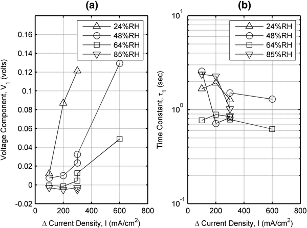
The parameters in the three-term model can be related to changes in operating conditions, such as current step size and reactant gas humidity. Figure
9
shows the first parameters,
V1
and
τ1
, plotted against the current step-up (
I2-I1
). Data for the largest current step at 85 % RH are excluded due to suspected flooding. The amplitude increases with both the size of the current step and the dryness of the reactant gases.
V1
is positive for the lower RH, serving to lessen the undershoot. It becomes small and negative, contributing to undershoot, with higher RH. The time constant
τ1
is essentially scattered around 1 s. Many of the outliers are points where
V1
indicates small amplitude; hence the time constant cannot be estimated accurately.
Fig. 9
Fit parameters for 80 °C current step increase data.
a
Amplitude
V1
;
b
time constant
τ1
The second parameter pair,
V2
and
τ2
, exhibited a similar trend. Figure
10
shows a linear relationship between
V2
and
I2
Δ
Ru
. The coefficient of determination is 0.91; in this case.
V2
increases with both the size of the current step and the dryness of the reactant gases. It is negative, representing undershoot in the voltage recovery. The low-humidity data (24 % RH) has time constant
τ2
that follows the time constant of cell ohmic resistance
τR
. The high-humidity data did not show a resistance change; a measurement of
τR
was not possible. Amplitude
V2
was correspondingly very small. Low-humidity voltage response has typically been associated with resistance changes, and component
V2
has a time constant
τ2
similar to the resistance measurement. Consider Eq. (
2
) which includes both membrane and catalyst layer protonic resistances.
Fig. 10
Fit parameter
V2
plotted against resistance change for low- to mid-humidity (+)step increase data
The third parameter pair,
V3
and
τ3
, could be correlated to changes of the rate of heat generation, per unit area, in the MEA. The amplitude
V3
is significantly greater with dry reactant inputs and varies monotonously with the final current step. The time constant
τ3
is 30–150 s and rises with reactant gas humidity. Wu [
34
] suggested that the effective heat capacity of the membrane contains contributions from both the dry membrane and its water content. Figure
11
shows that
V3
increases with changing heat generation,
ΔQ˙
,between the initial and final states. The rate of MEA heat generation in either state is [
35
]:
Q˙=I1.25-V
Fig. 11
Fit parameter
V3
plotted against change in heat generation for low- to mid-humidity data:
a
(+) current step,
b
(−) current step
Problems of mathematical ill-conditioning are not thought to be responsible for the data scatter, because the third time constant was significantly removed from the first two in all measurements. The greatest outliers from the trend line are the exceedingly dry measurements of group C1, which have the largest
V3
amplitudes. These most violate the implicit assumption in Eq. (
6
) that there is a single sudden change in levels of heat generation pre-step and post-step. The automatic action of the unit’s temperature control system, attempting to compensate, may have also added scatter to all readings. The best parabolic fits to the data are: −
V3
= 0.001 + 0.042Q − 0.010Q
2
and
V3
= 0.003 – 0.052Q – 0.044Q
2
, with correlation coefficients (
r
) of 0.77 and 0.93, respectively.
Discussion of timescales
Table
5
summarizes transient processes and timescales known from previous works. Several are too fast to measure on a 0.1 s resolution. There are five (5) key MEA transients. Electric double-layer charging is too rapid to be seen here. The water diffusion and hydration processes influence the time-varying voltage through resistance terms that change with membrane-phase water content. The last thermal value refers to the time constant of MEA temperature changes due to step changes in load. Time constants of transient response that can be measured (with a sampling rate of 10 Hz) include
τm,d
,
τRCLH+
,
τm,h
, and
τT
. The numbers 1–3 indicate the time constant values from the present study.
Table 5
Timescales of PEMFC processes that contribute to transient response
Gas-phase transient processes
τk
Gas diffusion through GDL media [10, 15, 20]
0.01 s
τgt
Gas transients of flow path [15]
0.1–0.2 s
Multiphase transient processes
τm-p
Liquid water accumulation [18, 36]
3 min
Transient processes of the MEA
τdl, τeod
Charging of electric double layer [18, 37]
0.2 μs
τm,d
Water diffusion across membrane [21]
0.2–0.8 s
τRCLH+1
Hydration—protonic resistance in catalyst layers [21]
1 s
τm,h2
Hydration—membrane protonic resistance [20]
5–20 s
τT3
Thermal [7, 34]
40–120 s
The typical resistance transient displays timescales
τm,d
and
τm,h
in its measurement of
(Re-+RmH+)
.
τm,d
indicates the amount of time post-current step for water imbalances through the membrane thickness to equilibrate: back diffusion occurs, anode side water content levels normalize, and membrane conductivity improves. Wang et al. [
21
] proposed the equation:
τm,d=δmem2Dmeff.
The hydration time constant
τm,h
reflects the time required for the MEA to gain or lose water content [
20
]. It was given at ~5–20 s, in line with
τR
measured here.
Voltage transients can be examined with a 0-dimensional model equation:
V=Voc-ηact⏟τ3-ηmt⏟τ1-i(Re-+RmemH++RaclH++RcclH+⏟τ1⏟τ2).
The cell voltage (
V
) is expressed in terms of the open-circuit voltage (
Voc
), and various losses. The activation overpotential (
ηact
) drives both the anode and cathode reactions; both are commonly assumed to follow Butler–Vollmer kinetics. This term has been assumed to remain constant with current throughout the transient event of voltage recovery [
18
]. It will change with catalyst layer temperature, however [
7
]. Fuel cell inner-component temperatures have been observed to vary with first-order response characteristic due to varied step inputs, for example, in SOFC devices [
38
]. The third component
V3
,
τ3
matches
τT
estimates at 40–120 s. Presumably, activation overpotential (
ηact
) changes due to temperature variations occurring at this time constant. Ionomeric-phase conductivity also has temperature dependence, potentially imparting a change in the resistance terms. Direct in situ temperature measurements have shown a linear temperature rise of the cathode catalyst layer (CCL), above the end-plate or current collector, of 0 °C to 5–7 °C, as current density increased from 0 to 1 A/cm
2
[
39
,
40
]. This 3 °C temperature rise from a cell block temperature between (50–80 °C) can be combined with the long-established conductivity relationship [
41
] to yield 3 % conductivity change. At a post-step current of 0.5 A/cm
2
with total ionomeric phase resistance of 0.090 Ω cm
2
, the change in voltage caused by this temperature-induced resistance change is only 1.3 mV. Hence, no significant
τ3
component is seen in the ohmic resistance measurement, and
τ3
is not indicated as affecting the catalyst layer resistances in Eq. (
8
).
The first component
V1
,
τ1
also matches the reported value of
τRCLH+
at ~1 s [
21
]. The catalyst layer resistances
(RaclH++RcclH+)
vary with time and contribute to cell dynamic response, particularly in the low-humidity case. Temporary flooding of the cathode catalyst layer has been suggested as an explanation of the 1 s delay observed in voltage recovery. If flooding was causing this delay, they would become more severe, or of longer duration, with increasing humidity of the cathode gas at the inlet. Measurements indicate the opposite actually occurs. Figure
12
shows measurements at 80 °C and four incrementally varying humidity levels for a 100–400 mA/cm
2
current step. The higher humidity measurements have been vertically shifted only for purposes of clarity. Delay is greatest where humidity is lowest, and delay is effectively suppressed by increasing humidity levels. Table
6
shows the first fit parameters and the observed delay in voltage response. The delay is greatest at low humidity, where amplitude
V1
is positive. At 85 % RH, amplitude
V1
becomes negative.
Fig. 12
Measurements of current step C1–C4[c+] from 0.1 to 0.4 A/cm
2
at 80 °C and variable %RH
Table 6
Variation of fit parameters
V
1,
τ
1, and delay in current step measurements C1–C4[c+] from 0.1 to 0.4 A/cm
2
at 80 °C and variable %RH
Humidity (RH)
V1 (v)
τ1 (s)
Delay (s)
24
0.121
1.27
2.5
48
0.023
0.82
1.5
64
0.004
0.84
1.1
85
−0.003
1.02
0.3
Conclusions
Dynamic responses of a typical single-cell PEMFC with a thin MEA to step changes in current load have been studied experimentally. Operating conditions were simplified to use excess stoichiometry and avoid water accumulation. Resistance and voltage transient responses are examined. These transient responses were well fitted by mono-exponential functions for the resistance and tri-exponential functions for the voltage. Previous studies have mostly used non-physical “black box” models to estimate dynamic response to step changes. The dynamic model’s optimal fitted parameters would change somewhat with operating conditions. With the tri-exponential model, a strategy which incorporates variable-fitted parameters might offer improved results. This work showed how a very simplified understanding of the physics of the MEA can explain some of the variations in amplitudes and timescales. The first component varies with temperature, humidity and current step size, at the fixed stoichiometry employed here. The second component showed amplitude variations, which correlate to ohmic resistance changes, from membrane hydration occurring during the current step. The third component is consistent with variable MEA heat generation, impacting the temperature-dependent activation losses in the cathode.
Acknowledgments
The authors wish to thank Dr. Kevin Cooper for his advice on the use of the fuel cell test system. The support of the National Science Foundation Marine Engineering Scholarship/Fellowship is gratefully acknowledged.
References
Wang et al. (2011) A review of polymer electrolyte membrane fuel cells: technology, applications, and needs on fundamental research 88(4) (pp. 981-1007) 10.1016/j.apenergy.2010.09.030
Unknown ()
Meiler et al. (2008) Dynamic fuel cell stack model for real-time simulation based on system identification 176(2) (pp. 523-528) 10.1016/j.jpowsour.2007.08.051
Hamelin et al. (2001) Dynamic behavior of a PEM fuel cell stack for stationary applications 26(6) (pp. 625-629) 10.1016/S0360-3199(00)00121-X
Yu and Ziegler (2006) Transient behavior of a proton exchange membrane fuel cell under dry operation 153(3) (pp. A570-A575) 10.1149/1.2162450
Hou (2011) A study on polarization hysteresis in PEM fuel cells by galvanostatic step sweep 36(12) (pp. 7199-7206) 10.1016/j.ijhydene.2011.03.059
Pathapati et al. (2005) A new dynamic model for predicting transient phenomena in a PEM fuel cell system 30(1) (pp. 1-22) 10.1016/j.renene.2004.05.001
Yan et al. (2006) Steady state and dynamic performance of proton exchange membrane fuel cells (PEMFCs) under various operating conditions and load changes 161(1) (pp. 492-502) 10.1016/j.jpowsour.2006.03.077
Kim and Min (2008) Experimental investigation of dynamic responses of a transparent PEM fuel cell to step changes in cell current density with operating temperature 22(11) (pp. 2274-2285) 10.1007/s12206-008-0702-4
Cho et al. (2008) Transient response of a unit proton-exchange membrane fuel cell under various operating conditions 185(1) (pp. 118-128) 10.1016/j.jpowsour.2008.06.073
Cho et al. (2011) Analysis of transient response of a unit proton-exchange membrane fuel cell with a degraded gas diffusion layer 36(10) (pp. 6090-6098) 10.1016/j.ijhydene.2011.02.060
Loo et al. (2010) Characterization of the dynamic response of proton exchange membrane fuel cells—a numerical study 35(21) (pp. 11861-11877) 10.1016/j.ijhydene.2010.08.071
Takaichi et al. (2007) Response of specific resistance distribution in electrolyte membrane to load change at PEFC operation 154(12) (pp. B1373-B1377) 10.1149/1.2794293
Moçotéguy et al. (2014) Influence of ageing on the dynamic behaviour and the electrochemical characteristics of a 500 We PEMFC stack 39(19) (pp. 10230-10244) 10.1016/j.ijhydene.2014.04.132
Kim et al. (2004) The effect of stoichiometry on dynamic behavior of a proton exchange membrane fuel cell (PEMFC) during load change 135(1–2) (pp. 110-121) 10.1016/j.jpowsour.2004.03.060
Kim et al. (2004) The effect of reservoirs and fuel dilution on the dynamic behavior of a PEMFC 137(1) (pp. 43-52) 10.1016/j.jpowsour.2004.05.035
Meiler et al. (2009) Nonlinear empirical model of gas humidity-related voltage dynamics of a polymer-electrolyte-membrane fuel cell stack 190(1) (pp. 56-63) 10.1016/j.jpowsour.2008.08.029
Hussaini and Wang (2009) Transients of water distribution and transport in PEM fuel cells 156(12) (pp. B1394-B1400) 10.1149/1.3236646
Um et al. (2000) Computational fluid dynamics modeling of proton exchange membrane fuel cells 147(12) (pp. 4485-4493) 10.1149/1.1394090
Wang and Wang (2005) Transient analysis of polymer electrolyte fuel cells 50(6) (pp. 1307-1315) 10.1016/j.electacta.2004.08.022
Wang and Wang (2006) Dynamics of polymer electrolyte fuel cells undergoing load changes 51(19) (pp. 3924-3933) 10.1016/j.electacta.2005.11.005
Ye and Wang (2007) Measurement of water transport properties through membrane-electrode assemblies 154(7) (pp. B676-B682) 10.1149/1.2737379
Unknown ()
Weydahl et al. (2008) Effect of gas composition and gas utilisation on the dynamic response of a proton exchange membrane fuel cell 180(2) (pp. 808-813) 10.1016/j.jpowsour.2008.01.037
Neyerlin et al. (2007) Cathode catalyst utilization for the ORR in a PEMFC 154(2) (pp. B279-B287) 10.1149/1.2400626
Unknown ()
Cornell and Berger (1987) Factors that influence the value of the coefficient of determination in simple linear and nonlinear regression models (pp. 63-70) 10.1094/Phyto-77-63
Spiess and Neumeyer (2010) An evaluation of R2 as an inadequate measure for nonlinear models in pharmacological and biochemical research: a Monte Carlo approach 10(1) 10.1186/1471-2210-10-6
Unknown ()
Yamaoka et al. (1978) Application of Akaike’s information criterion (AIC) in the evaluation of linear pharmacokinetic equations 6(2) (pp. 165-175) 10.1007/BF01117450
Wu et al. (2007) Non-isothermal transient modeling of water transport in PEM fuel cells 165(1) (pp. 232-243) 10.1016/j.jpowsour.2006.11.061
Unknown ()
Wang and Wang (2007) Two-phase transients of polymer electrolyte fuel cells 154(7) (pp. B636-B643) 10.1149/1.2734076
Wang (2004) Fundamental models for fuel cell engineering 104(10) (pp. 4727-4766) 10.1021/cr020718s
Barelli et al. (2014) SOFC thermal transients: modeling by application of experimental system identification techniques 14(1) (pp. 107-122) 10.1002/fuce.201300164
Unknown ()
Zhang et al. (2010) Simultaneous measurement of current and temperature distributions in a proton exchange membrane fuel cell 195(11) (pp. 3597-3604) 10.1016/j.jpowsour.2009.12.016
Springer et al. (1991) Polymer electrolyte fuel cell model 138(8) (pp. 2334-2342) 10.1149/1.2085971