Engineering Department “Enzo Ferrari”, University of Modena and Reggio Emilia, Modena, 41125, IT
Abstract
Urban areas usually experience higher temperatures when compared to their rural surroundings. Several studies underlined that specific urban conditions are strictly connected with the Urban heat island (UHI) phenomenon, which consists in the environmental overheating related to anthropic activities. As a matter of fact, urban areas, characterized by massive constructions that reduce local vegetation coverage, are subject to the absorption of a great amount of solar radiation (short wave) which is only partially released into the atmosphere by radiation in the thermal infrared (long wave). On the contrary, green areas and rural environments in general show a reduced UHI effect, that is lower air temperatures, due to evapo-transpiration fluxes. Several studies demonstrate that urban microclimate affects buildings’ energy consumption and calculations based on typical meteorological year could misestimate their actual energy consumption. In this study, two different sets of meteorological data are used for the calculation of the heating and cooling energy needs of an existing university building. The building is modeled using TRNSYS v.17 software. The first set of data was collected by a weather station located in the city center of Modena, while the second set of data was collected by another station, located in the surrounding area of the city, near to the studied building. The influence of the different meteorological situations described by the two weather stations are analyzed and assumed to be representative of the UHI effect. Furthermore, the effects of UHI mitigation strategies on the building energy needs are evaluated and discussed.
Introduction
Urban areas usually experience higher temperatures when compared to their rural surroundings. Several studies [
1
,
2
] underlined that specific urban conditions are strictly connected with the Urban heat island (UHI) phenomenon, which consists in the environmental overheating related to anthropic activities. This effect is usually quantified referring to the urban heat island intensity, which is defined as the maximum difference between urban and surrounding areas temperatures.
Buildings, roads, and other constructions in urban areas absorb heat during the day and re-emit it after sunset, creating high temperature differences between urban and rural areas [
3
].
Many causes bring to higher temperatures in urbanized environment, such as anthropogenic heat, excess of heat stored by construction materials, decreased long-wave radiation losses from urban areas, lack of vegetation and reduced evapo-transpiration processes, reduction of wind speed and consequent reduced convective heat removal from urban surfaces to the atmosphere.
Several studies [
4
–
6
] demonstrate that urban microclimate affects buildings energy consumption. Indeed, building energy consumption in urban areas is not only determined by envelope and equipment features. Urban heat island and the immediate surrounding can affect the energy performance of buildings located in densely built areas. These buildings, besides rural or suburban ones, undergo several UHI effects such as higher external air temperatures, lower wind speeds and reduced energy losses during the night period. These effects have a significant impact especially on cooling energy consumption [
7
].
Moreover, most of the studies consider only the energy consumption during the summer period, and there is still a lack of evaluation of the effects of urban microclimate on the annual energy consumption.
Kikegawa et al. [
8
] developed a simulation model that can describe relations between summer weather conditions in urban contexts and building cooling energy needs. They found that the peak-time cooling electric power demand in a central business district in Tokyo could decrease up to 6 % with a reduction of the outdoor air temperature by more than 1 °C.
According to Santamouris et al. [
5
], the cooling load of urban buildings may increase twofold and the peak cooling electricity load may be tripled by the UHI effects noticed in Athens. Moreover, during winter time, results have shown that urban buildings’ heating energy needs may decrease by about 30–50 % compared to rural or suburban buildings.
Energy needs of urban buildings can be assessed in wide spatial and temporal ranges. The major scale considers phenomena such as UHI effect. The effect on a single building can also be analyzed. In this case the energy load of the building is assessed using energy simulation models and appropriate boundary conditions have to be defined. By supplying the simulation with modified meteorological data, heat island effects can be properly described [
9
].
In addition, it has been found that calculations based on typical meteorological year could misestimate the actual energy consumption. The influence of actual weather data is generally disregarded in the energy performance calculation. However, to consider the actual interactions between indoor and outdoor environments, the use of real weather data in building energy simulations is required [
10
]. Moreover, to identify urban heat island features in the considered area, a spatial characterization of ambient temperature is required. Nevertheless, the reference weather station is generally located in a sparsely built area. Both urban and rural climatic data are not frequently used to get the real assessment of the impact of UHI on building energy needs [
11
].
Different studies [
11
,
12
] have confirmed the impact of UHI on the energy needs of buildings, using measured air temperature data as input to an energy simulation model to assess heating and cooling load of a building positioned at different locations within the urban area.
Concerning UHI countermeasures, most studies evaluate only the effects on cooling energy consumption in summer, even though UHI mitigation may increase heating energy consumption in winter [
6
,
13
,
14
].
The present study is aimed at considering the real weather data effects on the thermal behavior of a building. These effects are evaluated for different seasons and locations, stressing out the consequences of both real climate events and UHI phenomenon. The assessment of the energy needs of the reference building is achieved in a comparative way, counting on the use of weather data collected from urban and suburban stations. In this study, two different sets of actual meteorological data [
15
,
16
] are used for the calculation of the annual energy needs of an existing university building. UHI countermeasure effects on energy needs are also assessed, both in summer and in winter period.
Materials and methods
Energy modeling and calculation
In this study the energy needs of an existing university building are calculated for both heating and cooling periods. The heating period extends from October 15 to April 15, while the cooling period extends from June 1 to September 15.
The annual energy needs of the building are determined by simulations carried out using the TRNSYS 17 [
17
] dynamic thermal modeling software.
TRNSYS is a deterministic building simulation program. Like other similar codes, such as DOE-2, ESP-r or EnergyPlus, it simulates the thermal performance of buildings and plants according to the input data about building envelope, HVAC systems, indoor gains and weather. All the physical components of the thermal energy system are represented by FORTRAN subroutines, combined into an executable file which describes their connections [
18
]. From the given set of input data, expressed as explicit time functions, the simulation predicts the building plant system behavior. Driving forces are modeled using a time discretization. The time resolution of available weather data determines the sampling time-step, usually of 1 h [
19
].
In particular, TRNSYS calculates transient heat conduction through multi-layer envelope components using the transfer function method (TFM), recommended by ASHRAE as one of the most accurate methods to calculate time-variable heat loads [
20
]. Formerly introduced by Mitalas [
21
], TFM describes the thermal behavior of building envelopes using few numerical coefficients. The method, using
Z
-transforms, solves the equation system that describes the heat transfer in a multi-layered wall.
Z
-transform is a mathematical operator widely used by simulations dealing with discrete signals in the time domain, such as climatic data. The TFM considers each component of the thermal energy system as a black box: the transfer function analyzes an input signal and carries out an output signal [
17
].
The simulation engine solves the system of algebraic and differential equations that represents the whole energy system. The results obtained by simulations analyzed in this study are winter and summer energy demands and external surface temperature profiles.
In this study, two different sets of meteorological data are used for the calculation of the heating and cooling needs of the university building. The first set of data was collected by a weather station located downtown Modena, while the second set of data was collected by another station, located in the surrounding area of the city, near to the studied building.
These weather stations are owned by the Geophysical Observatory of the University of Modena and Reggio Emilia and the available half-hourly weather data include global radiation on horizontal, dry bulb temperature, wind speed and relative humidity.
UHI countermeasure effects on energy needs are assessed by considering a “cool” coating with high solar reflectance on the roof (solar absorptance
αsol
= 0.25) and on the opaque vertical surfaces (
αsol
= 0.25).
Building description
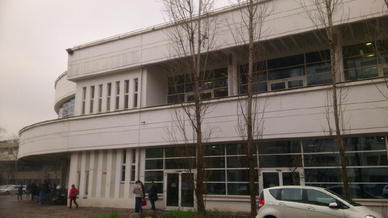
In this study, the Interdepartmental Scientific Library (ISL) of the University of Modena and Reggio Emilia has been selected for the comparative analysis.
The two-storey building is composed by the main reading room, of about 12 m height, several offices, two archives, meeting and technical rooms (see Figs.
1
and
2
). Table
1
summarizes the most important geometrical characteristics of the selected building.
Fig. 1
Plan of the building
Table 1
Main geometrical characteristics of the building
Floor surface (m2)
2,200
Opaque vertical surfaces (m2)
1,925
Transparent surfaces (m2)
718
Gross volume (m2)
1,8313
The building is located in the city of Modena; it was built in 1998. The library has concrete and light-insulated walls [
Uw
= 0.52 W/(m
2
K)], double-glazed windows [
Ug
= 2.83 W/(m
2
K),
g
= 0.45], and a non-insulated flat roof [
Ur
= 1.32 W/(m
2
K)] with north-oriented vertical windows in a saw-toothed roof (see Tables
2
,
3
).
Fig. 2
View of north façade of the building
Table 2
Thermal transmittance of the building envelope
Description
U [W/(m2K)]
Opaque vertical surfaces
0.52
Roof
1.32
Transparent surfaces
2.83
Table 3
Layers and thermal properties of the building envelope
Layers
S (m)
λ [W/(mK)]
c [kJ/(kgK)]
ρ (kg/m3)
Opaque vertical surfaces
Concrete panel
0.24
0.51
1
1,400
Insulation
0.05
0.04
1.4
10
Gypsum plaster
0.01
0.35
1
1,200
U [W/(m2K)]
0.52
Roof
Bitumen waterproof coating
–
0.17
1
1,200
Concrete slab
0.30
0.51
1
1,400
Gypsum plaster
0.01
0.35
1
1,200
U [W/(m2K)]
1.32
Description of meteorological data
The historical atmospheric temperatures are available for the urban area weather station, where the University Geophysical Observatory is collecting data since 1830 [
22
].
Modena time series show a temperature increase trend which is higher than the global one, according with other weather stations of the Emilia Romagna Region [
22
]. In particular, Modena is characterized by a more extreme climate, with an increasing of extreme events, especially hotter summer and heat waves, like the one known as “summer 2003 in Europe” [
23
]. Considering the city of Modena, 2012 has been characterized by several heat waves [
16
]. It is also possible to observe that there are significant differences between the two meteorological years, especially during spring and summer period.
Winters are generally milder than the past, but 2012 has been characterized by a very rigid winter in Emilia, with strong cold air outbreak with many “ice days” (both
Tmin
and
Tmax
below 0 °C) and heavy snowfall.
In Fig.
3
the monthly average atmospheric temperatures for 2011 and 2012 are compared with the 30-year climate data (1981–2010). One can observe that the selected years are characterized by monthly average atmospheric temperatures that are generally higher than the historical ones, according to the climate indicators [
24
].
Fig. 3
Comparison between monthly average atmospheric temperature in 2011 and 2012 and historical data (1981–2010 period)
In Fig.
4
the average monthly atmospheric temperatures for the urban and suburban areas of Modena are compared. The results show that the urban monthly average temperatures are always higher than the suburban ones, and an average 1.4 °C temperature difference is found.
Fig. 4
Average monthly atmospheric temperature in 2012: comparison between urban and suburban area weather stations.
a
2011,
b
2012
In Figs.
5
and
6
the half-hourly atmospheric temperature data are presented for the three coldest days of 2012 (5th–7th of February). It is possible to observe that the higher temperature differences between urban and suburban areas are found during the nocturnal period, where values of around 6 °C are reached. The same situation is observed during the hottest days of 2012 (21st–23rd of August).
Fig. 5
Half-hourly atmospheric temperature profiles in the urban and suburban areas: 5th–7th February 2012
Fig. 6
Half-hourly atmospheric temperature profiles in the urban and suburban areas: 21st–23rd August 2012
Results and discussion
Simulations have been performed for the base-case model (Case 0) and the case with the application of cool coating on roof and opaque vertical surfaces (
αsol
= 0.25) (Case 1).
The hourly indoor air temperature measurements were used to analyze the discrepancies between simulated and actual building energy performance. The measurements were available for three different periods: February, July and September 2012. The simulated indoor air temperatures of the base-case model were used for the comparison. Due to the actual building’s location, the meteorological data of the suburban area were used for the base-case model.
Statistical analyses were performed by calculating the mean bias error (MBE), the root mean square error (RMSE) and the Pearson’s Index r. The results of the error analysis procedure are outlined in Table
4
.
Table 4
Statistical analysis
MBE
RMSE
Pearson (r)
0.21
0.83
0.97
As reported in Table
4
, MBE results show a slight overestimation of the predicted temperature with respect to the actual data. Considering the MBE error compensation, this index was not considered exhaustive to evaluate the reliability of the model and both RMSE and Pearson’s index were also investigated. The results show that the selected indexes are in agreement with the tolerance range (see Table
4
) and the model is considered representative of the actual energy performance.
To assess the overall primary energy needs, the efficiency of the system was taken into account. Considering the heating system, an overall system efficiency of 73 % is considered. On the other hand, for the cooling system an average energy efficiency ratio (EER) of 2 is considered.
Tables
5
and
6
show that annual energy needs are lower when the cooling coating is applied on the roof and on the opaque vertical surfaces (see Fig.
7
).
Table 5
Energy needs and primary energy required by the reference building (MWh)
Period
Weather station location
2011
2012
Case 0
Case 1
Case 0
Case 1
Energy need
Summer
Urban area
99
83
112
94
Suburban area
91
75
103
86
Winter
Urban area
38
43
45
48
Suburban area
48
53
55
60
Year
Urban area
137
126
156
143
Suburban area
139
128
158
146
Primary energy
Summer
Urban area
130
108
146
123
Suburban area
120
98
135
112
Winter
Urban area
52
59
61
66
Suburban area
65
73
76
82
Year
Urban area
182
168
208
190
Suburban area
185
171
211
194
Table 6
Results for case 1: variation of energy needs compared to Case 0
Description
Weather station location
2011 (%)
2012 (%)
Summer
Variation of energy needs compared to case 0
Urban area
−16
−16
Suburban area
−18
−17
Winter
Variation of energy needs compared to case 0
Urban area
13
8
Suburban area
11
9
Fig. 7
Energy need in summer (
a
) and winter (
b
) period
Figure
8
shows a comparison between the four meteorological data for Case 0 and Case 1. The results show higher summer needs in 2012 (increase of 13 % compared to 2011), due to several heat waves.
Fig. 8
Energy need relative to different meteorological data. Summer period (
a
) and winter period (
b
)
Simulations have been carried out with the two weather stations’ meteorological data. The comparison of the two set of simulation results underlines the UHI effects. As shown in Table
7
, summer energy needs of the building located in urban area are around 10 % higher than the energy needs of the building located in suburban area.
Table 7
Variation of energy needs and primary energy required by the building located in suburban area compared to the building located in urban area
2011
2012
Case 0 (%)
Case 1 (%)
Case 0 (%)
Case 1 (%)
Variation of energy needs
Summer
−8
−10
−8
−10
Winter
20
19
19
19
Year
1
2
1
2
Variation of primary energy
Summer
−8
−10
−8
−10
Winter
20
19
19
19
Year
2
2
1
2
On the other hand, in winter period energy needs’ values related to the suburban area are about 15 % higher.
The results summarized in Table
7
show that the overall year energy needs increase up to 2 % in the absence of UHI effect.
Table
8
shows the influence of UHI on CO
2
equivalent emissions. Due to the increase of the cooling energy demand, CO
2
equivalent annual emissions rise up to 7 % in presence of the UHI. The results have been obtained using carbon dioxide emission coefficients for natural gas (55 g CO
2
eq/MJ) and electricity (150.1 g CO
2
eq/MJ) [
25
,
26
].
Table 8
CO
2
equivalent emissions (kg)
Weather station location
2011
2012
Case 0
Case 1
Case 0
Case 1
Summer
Urban area
153
128
172
145
Suburban area
141
116
159
132
Winter
Urban area
10
12
12
13
Suburban area
13
14
15
16
Year
Urban area
163
139
185
158
Suburban area
154
130
174
149
Variation of CO2 equivalent emissions of the building located in suburban area compared to the building located in urban area
−5 %
−6 %
−7 %
−6 %
In addition, a significant reduction of annual CO
2
emissions due to the application of cool coating is found in Table
9
. The decrease of up to 15 % demonstrates the positive effect of UHI countermeasures on the reduction of greenhouse gas emissions.
Table 9
Variation of CO
2
equivalent emissions of the building with cool coatings referred to the building without cool coatings
Weather station location
2011 (%)
2012 (%)
Year
Urban area
−14
−14
Suburban area
−15
−15
In addition, three representative days of the summer period are analyzed in Fig.
9
. The results underline the higher cooling energy need presented by Case 0 compared to Case 1, as well as the higher cooling need presented with the urban area weather data compared with the suburban ones.
Fig. 9
Energy need on 16th–18th July 2012. Urban and suburban weather data
Also for the winter period three representative days are analyzed. The results (Fig.
10
) show a slight increase of energy needs, about 4 %, due to the application of cool coating, compared to the base case. Moreover, the comparison between energy needs of the building located in urban area and the building located in the suburban area presents a decrease of an average of 25 %.
Fig. 10
Energy need on 8th–10th January 2012. Urban area and suburban area weather data
External roof surface temperature profiles are analyzed for the different simulation cases, considering three representative summer days of 2012.
The analysis demonstrates that the external temperature of roof surface achieves high values, up to 55 °C in Case 0 (see Fig.
11
). By the application of cool coating on the roof surface, peaks decrease to 35 °C. In general, the application of cool roof coating allows one to achieve an average daily decrease of 6 °C on roof external surface, reducing significantly its overheating.
Fig. 11
Atmospheric temperature and external roof surface temperature on 16th–18th July 2012.
a
Urban area weather data,
b
suburban area weather data
The comparison between the results obtained using the data from the two different weather stations (Fig.
12
) underlines that the most significant UHI effects occur during the night time (from 7:00 PM to 6:00 AM). On the other hand, during daytime, solar irradiation reaches highest values and the external roof surface temperature does not change significantly from urban to suburban area.
Fig. 12
Atmospheric temperature and external roof surface temperature on 16th–18th July 2012;
a
case 0,
b
case 1
Conclusions
In this study, the influence of actual weather data has been considered in the annual energy performance calculation of an existing building. The simulations carried out with the meteorological data from two different weather stations demonstrate the effects of UHI on building energy needs.
More studies evaluated the effects of UHI and the relative mitigation measures only on cooling energy consumption, even though UHI mitigation may increase heating energy consumption in winter.
The novelty represented by this study consists in considering UHI mitigation effects on energy needs both in winter and summer period. The outcomes show that energy needs of the reference building are influenced by UHI effect. In presence of the UHI effect, net annual cooling and heating energy use slightly decreases. The result is consistent with other studies [
5
]. On the other hand, UHI effects on reference building energy consumption lead to the rise of CO
2
equivalent annual emissions of up to 7 %.
In addition, the results show that UHI mitigation could achieve significant energy savings on cooling energy needs in summer; however, they may slightly increase heating energy need in winter. In the considered case, heating and cooling energy needs have been converted in primary energy, showing that the balance throughout the whole year period is positive and encouraging towards the usage of cool coating.
Moreover, this study demonstrates that, by the application of cool coating on the roof surface, peaks of the external temperature of roof surface decrease by about 6 °C during daytime, avoiding its overheating.
The UHI effects on other building types, such as residential or commercial buildings, will also be investigated in the future.
Author contributions
SM and CL carried out the computational simulations and drafted the manuscript. LL, AM and ST provided technical guidance and critical review of the manuscript. All authors read and approved the final manuscript.
Acknowledgements
The authors would like to acknowledge the Energy Efficiency Laboratory (EELab) of the Engineering Department of the University of Modena and Reggio Emilia. The Energy Efficiency Laboratory is the lead partner of the MAIN Project partially funded by Programme MED (EU). The project is aimed at intervening in any chain cycle for the use of the smart materials here called MAIN, the set of cool roof and cool pavement solutions.
Conflict of interest
The authors declare that they have no competing interest.
References
Kolokotroni and Giridharan (2008) Urban heat island intensity in London: an investigation of the impact of physical characteristics on changes in outdoor air temperature during summer 82(11) (pp. 986-998) 10.1016/j.solener.2008.05.004
Schwarz et al. (2012) Relationship of land surface and air temperatures and its implications for quantifying urban heat island indicators—an application for the city of Leipzig (Germany) (pp. 693-704) 10.1016/j.ecolind.2012.01.001
Shahmohamadi et al. (2011) The impact of anthropogenic heat on formation of urban heat island and energy consumption balance (pp. 1-9) 10.1155/2011/497524
Unknown ()
Santamouris et al. (2001) On the impact of urban climate on the energy consumption of buildings 70(3) (pp. 201-216) 10.1016/S0038-092X(00)00095-5
Ihara et al. (2008) Changes in year-round air temperature and annual energy consumption in office building areas by urban heat-island countermeasures and energy-saving measures 85(1) (pp. 12-25) 10.1016/j.apenergy.2007.06.012
Kolokotroni et al. (2006) The effect of the London urban heat island on building summer cooling demand and night ventilation strategies 80(4) (pp. 383-392) 10.1016/j.solener.2005.03.010
Kikegawa et al. (2004) Development of a numerical simulation system toward comprehensive assessments of urban warming countermeasures including their impacts upon the urban buildings’ energy-demands 45(3) (pp. 449-466)
Moonen et al. (2012) Urban Physics: effect of the micro-climate on comfort, health and energy demand 1(3) (pp. 197-228) 10.1016/j.foar.2012.05.002
He et al. (2009) A numerical simulation tool for predicting the impact of outdoor thermal environment on building energy performance 86(9) (pp. 1596-1605) 10.1016/j.apenergy.2008.12.034
Santamouris (2014) On the energy impact of urban heat island and global warming on buildings (pp. 100-113) 10.1016/j.enbuild.2014.07.022
Kolokotroni et al. (2007) The London heat island and building cooling design 81(1) (pp. 102-110) 10.1016/j.solener.2006.06.005
Hirano and Fujita (2012) Evaluation of the impact of the urban heat island on residential and commercial energy consumption in Tokyo 37(1) (pp. 371-383) 10.1016/j.energy.2011.11.018
Pisello and Cotana (2014) The thermal effect of an innovative cool roof on residential buildings in Italy: results from 2 years of continuous monitoring (pp. 154-164) 10.1016/j.enbuild.2013.10.031
Lombroso (2011) Annuario delle osservazioni meteoclimatiche dell’anno 2011 registrate dall’Osservatorio Geofisico di Modena (pp. 5-25)
Lombroso (2012) Annuario delle osservazioni meteoclimatiche dell’anno 2012 registrate dall’Osservatorio Geofisico di Modena (pp. 5-25)
Unknown ()
Hong et al. (2000) Building simulation: an overview of developments and information sources 35(4) (pp. 347-361) 10.1016/S0360-1323(99)00023-2
Beccali et al. (2005) Is the transfer function method reliable in a European building context? A theoretical analysis and a case study in the south of Italy? 25(2–3) (pp. 341-357) 10.1016/j.applthermaleng.2004.06.010
Giaconia and Orioli (2000) On the reliability of ASHRAE conduction transfer function coefficients of walls 20(1) (pp. 21-47) 10.1016/S1359-4311(99)00005-8
Höglund et al. (1967) Surface temperatures and heat fluxes for flat roofs 2(1) (pp. 29-36) 10.1016/0007-3628(67)90005-9
Unknown ()
Schär et al. (2004) The role of increasing temperature variability in European summer heatwaves (pp. 332-336) 10.1038/nature02300