German Aerospace Center (DLR) Institute of Networked Energy Systems, Oldenburg, 26129, DE
Deutsche Gesellschaft Für Internationale Zusammenarbeit (GIZ) GmbH, New Delhi, 110029, IN
Solar Radiation Resource Assessment, National Institute of Wind Energy, Chennai, 600100, IN
Overspeed GmbH & Co. KG, Oldenburg, 26129, DE
Institute of Physics, Carl von Ossietzky University of Oldenburg, Oldenburg, 26111, DE
Abstract
Due to the steep rise in grid-connected solar Photovoltaic (PV) capacity and the intermittent nature of solar generation, accurate forecasts are becoming ever more essential for the secure and economic day-ahead scheduling of PV systems. The inherent uncertainty in Numerical Weather Prediction (NWP) forecasts and the limited availability of measured datasets for PV system modeling impacts the achievable day-ahead solar PV power forecast accuracy in regions like India. In this study, an operational day-ahead PV power forecast model chain is developed for a 250 MWp solar PV park located in Southern India using NWP-predicted Global Horizontal Irradiance (GHI) from the European Centre of Medium Range Weather Forecasts (ECMWF) and National Centre for Medium Range Weather Forecasting (NCMRWF) models. The performance of the Lorenz polynomial and a Neural Network (NN)-based bias correction method are benchmarked on a sliding window basis against ground-measured GHI for ten months. The usefulness of GHI transposition, even with uncertain monthly tilt values, is analyzed by comparing the Global Tilted Irradiance (GTI) and GHI forecasts with measured GTI for four months. A simple technique for back-calculating the virtual DC power is developed using the available aggregated AC power measurements and the inverter efficiency curve from a nearby plant with a similar rated inverter capacity. The AC power forecasts are validated against aggregated AC power measurements for six months. The ECMWF derived forecast outperforms the reference convex combination of climatology and persistence. The linear combination of ECMWF and NCMRWF derived AC forecasts showed the best result.
Introduction
The intermittent nature of solar resource poses a challenge in producing reliable generation forecasts for grid-connected solar Photovoltaic (PV) systems. As the initial bid or generation schedule needs to be provided on a day-ahead basis, accurate day-ahead predictions are essential for the financial security of PV plant owners. Grid operators of power systems with a high penetration of solar PV require these forecasts to ensure the maintenance of load-generation balance. Due to the ever-increasing emphasis on climate targets, as seen recently at the COP26, renewable electricity capacity is expected to surpass 4800 GW by 2026 [
1
]. According to the International Energy Agency (IEA), Solar PV is alone expected to account for half of all renewable power expansion worldwide from 2021 to 2026. India has the highest growth rate in renewable power capacity relative to the existing capacity [
1
]. As of August 2022, the nationwide installed capacity of grid-connected solar PV is 63 GW [
2
]. In a recent update to its Nationally Determined Contribution (NDC), the Indian Government has decided to reduce the emissions intensity of its GDP by 45% till 2030 [
3
]. Solar PV is expected to play a leading role in achieving its ambitious target. However, the data availability from these PV systems is often restricted to measurements of irradiance, module temperature, and inverter AC power output. To cope with the increasing demand for accurate solar PV forecasts, our forecast model chain is developed and benchmarked for Indian meteorological conditions with a limited availability of measured datasets from the site.
Solar irradiance forecasts from Numerical Weather Prediction (NWP) model produce accurate and reliable results for day-ahead and multiday-ahead forecast horizons [
4
,
5
–
6
]. In the subsequent steps, forecasted irradiance is converted into the PV power output using statistical, physical, or a combination of both models. Statistical and machine learning models are trained with past irradiance measurements, module and meteorological parameters, and the final PV power output to derive a direct relationship between them. The accuracy of such models depends on the available length of historical training data [
7
,
8
,
9
–
10
]. Alternatively, physical models are used for the transposition of Global Horizontal Irradiance (GHI) to Global Tilted Irradiance (GTI), modeling the DC power output as a function of GTI and PV module temperature, or modeling the inverter DC to AC power conversion efficiency in a stepwise manner [
11
,
12
], as shown in Fig.
1
. A hybrid combination of the physical and machine learning-based methods can also serve specific purposes, such as the removal of data points with curtailment before model training [
13
].
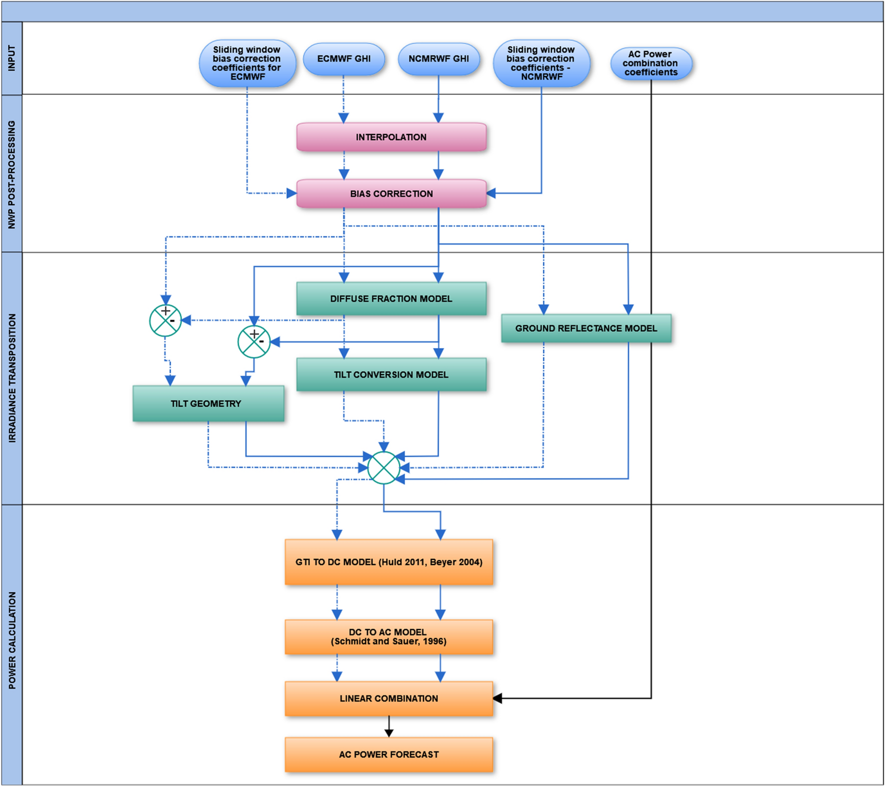
Fig. 1
Schematic of the forecasting model chain from NWP input (top) to final combined power forecast (bottom)
The NWP model output GHI needs to be temporally interpolated to match the time resolution of the generation schedule mandated by regulations [
14
,
15
]. An initial bias correction of the NWP modeled GHI is useful for the removal of systematic deviations and improves the accuracy of the predicted GHI. Various bias correction techniques using ground measurements are found in the literature, including polynomial functions [
14
,
16
,
17
], Kalman Filtering [
18
,
19
], and Neural Networks (NN) [
20
,
21
–
22
]. Methods for bias correction of NWP solar irradiance output using geostationary satellite data images are also reported [
23
]. Diffuse fraction and diffuse sky models transform forecasted GHI into GTI [
24
]. The diffuse fraction model splits the GHI into its beam and diffuse components [
25
,
26
–
27
]. This is usually achieved in the simplest case by modeling the diffuse fraction (ratio of the diffused irradiance to the global irradiance) as a function of the clearness index (ratio of the global irradiance to the top of the atmosphere irradiance). Advanced methods can use multiple astronomical and meteorological parameters as predictors [
29
,
30
–
31
]. GTI incident on the module and the cell temperature influence efficiency and, consequently, the DC power output. PV module efficiency can be modeled using detailed diode equivalent circuits [
32
,
33
] or as empirical functions of incident irradiance and cell temperature [
12
,
34
,
35
,
36
–
37
]. An increase in operating cell temperature beyond 25 °C has a negative impact on the electrical efficiency of PV modules, and the losses can be significant for regions like India [
38
,
39
–
40
]. Detailed inverter efficiency curves at different voltage levels can be obtained from the manufacturer’s data sheet [
41
]. The conversion efficiency of the module DC power output into AC power by the inverter can also be modeled in multiple ways: constant efficiency, polynomial efficiency curve, and voltage-dependent polynomial efficiency curves [
42
,
43
,
44
,
45
–
46
].
In this study, an operational day-ahead PV power forecast model is developed using a combination of the NWP datasets from the European Centre of Medium Range Weather Forecasts (ECMWF) and the National Centre for Medium Range Weather Forecasting (NCMRWF) models. Its components are benchmarked for a 250 MWp solar PV plant located in Southern India. In [
47
], the authors proposed using the Lorenz polynomial bias correction function as a reference for benchmarking newer methods. In [
48
], the authors validated the improvement in accuracy due to NN-based bias correction against ground-measured data from four stations located on the La Réunion Island. In [
22
], the authors developed an optimally configured NN-based corrective algorithm for NWP output GHI and validated it against ground measurements from two sites in southern Portugal. However, a benchmark of the NN-based technique against the Lorenz polynomial method is not shown. In this work, the accuracy of the two bias correction techniques is intercompared for ten months. [
7
] suggested that assuming a tilt value could be better than using the GHI directly in the case of irradiance transposition with an unknown module tilt. However, the validation of forecasted GTI obtained from an assumed tilt against ground measurements is lacking. Especially for situations where the module tilt is changed manually on a seasonal basis, with every readjustment cycle lasting multiple days, as in the case of the PV plant analyzed in this work. The utility of using even approximate module tilt values for irradiance transposition is shown in this study. In [
7
], the author studied the power output simulation of 16 PV plants for five data availability scenarios but did not consider the case in which the AC power output dataset is available while DC power is not. In the current analysis, DC power is back-calculated from the AC power due to the lack of the inverter DC side measurements. However, this situation is encountered quite frequently in India; therefore, the current work provides a practical solution for such cases. In [
48
], the authors implemented and tested a site-specific bias correction technique for NWP-based AC power forecasts across 23 PV sites in Finland. However, the method uses NWP forecast data from a single model and does not combine multiple NWP model outputs. In [
49
], the authors generated solar power forecasts from two different parameterizations of the same Weather Research and Forecasting (WRF) model and subsequently performed a linear combination of the two power forecasts. However, they did not use a reliable standard of reference, such as, the convex combination of persistence and climatology [
50
,
51
], for analyzing the utility of the forecasts.
This study has the following specific objectives: -
Benchmarking the performances of the Lorenz polynomial and Neural Network (NN)-based bias correction methods on a sliding window basis.
Validation of the benefit of using a GHI transposition model even with uncertain or approximate PV module tilt information.
Estimating DC power from aggregated AC power meter readings.
Development of an operational physical model chain for solar PV power forecast.
Analyzing the utility of AC power forecasts derived from ECMWF and NCMRWF against the reference convex combination of persistence and climatology.
Linear combination of the two AC power forecasts and validation of the improvement against the convex combination of persistence and climatology.
Data and methods
The forecast model chain is a collection of individual models that convert the GHI output from the NWP dataset into GTI at the PV module tilt and then finally into the plant AC power output by modeling each stage of energy conversion in the PV plant. A conceptual schematic of the model chain is shown in Fig.
1
.
Numerical weather prediction data
NWP datasets from ECMWF and the NCMRWF are used in this work. The ECMWF High Resolution Forecast (HRES) model runs twice daily at 00 and 12 UTC, and produces three hourly predictions up to three days ahead at a spatial resolution of 0.25˚ × 0.25˚. NCMRWF provides global, regional, deterministic and ensemble predictions. The deterministic global model is run twice daily at 00 and 12 UTC, and provides hourly forecast up to nine days ahead with a spatial resolution of 0.25° × 0.25°. Each global model’s 00 UTC run output is used for generating solar power forecasts in this analysis.
Solar radiation resource assessment network data
Quality controlled ground-measured irradiance data from the nearest Solar Radiation Resource Assessment (SRRA) station at Kadiri is also used in training the bias correction model. SRRA is a network of long-term solar radiation monitoring stations spread across 115 locations over India. These stations are equipped for sampling GHI, Diffuse Horizontal Irradiance (DHI), Direct Normal Irradiance (DNI), ambient temperature, humidity, wind speed, wind direction, rain accumulation and barometric pressure every second before averaging them over every one minute and recording them [
52
].
Power plant data
The test site shown in Fig.
2
consists of five 50 MWp blocks of solar PV plants co-located within the same Solar Park, with each block having a different module type, size and manufacturer. The module tilt angle of each block varies independently on a seasonal basis. An average monthly module tilt schedule for all blocks combined has been prepared (see Table
1
) from the approximate tilt change schedule obtained from site survey. Dynamic datasets from the power plant include time series measurements of GHI, GTI, PV module temperature and the aggregated AC power output of the park at an interval of 15 min. DC measurements from the inverter are not available. The irradiance measurements are quality controlled using the same checks as used for the SRRA stations [
53
]. These include the missing value test, tracking error test, minimum diffuse radiation test, coherence test, clear-sky test, maximum physical limit test and minimum physical limit test. The power measurements are quality-controlled using stuck value check, non-zero nighttime value check, maximum possible ramp check and physical limit check.
Fig. 2
Location of the power plant (Google earth image)
Table 1
Averaged tilt of the 5 individual blocks on a seasonal basis
Month Number
1
2
3
4
5
6
7
8
9
10
11
12
Module Tilt
27°
27°
9°
4°
4°
4°
4°
4°
6°
14°
23°
26°
Interpolation of numerical weather prediction data
The raw GHI predictions from NWP data are available only for a pre-defined number of grid points. The average of the predicted GHI at the four grid points closest to the center coordinate of the plant is computed. The average GHI can be subsequently interpolated to 15 min from its original hourly or three hourly resolution by using the clear sky index interpolation method [
14
,
15
]. Furthermore, in [
54
] it is shown that using a more intricate clear sky model does not necessarily imply better forecasts. The computationally simple model proposed in [
55
] is used in this analysis to compute clear sky indices
ktorig res
from the NWP output GHI dataset at the original temporal resolution, as shown in Eq.
1
. Clear sky indices
kt15min
in 15 min temporal resolution is derived by assuming that the original clear sky indices remain constant within each hourly or three hourly period depending on the actual time resolution of the NWP output. The 15-min resolution GHI dataset can be estimated, as shown in Eq.
2
.
ktorig res=GHINWPorig resGHIclear skyorig resGHINWP15min=kt15min·GHIclearsky15min
Bias correction of irradiance data from numerical weather prediction model
NWP models have a coarse resolution spanning a large area (grid cell), and a systematic bias in the prediction may be observed when compared with site-specific ground measurements of GHI. The mathematical expression for bias is shown in Eq.
3
. This is influenced by the local conditions at the site.
bias=GHINWP-GHImeas
Lorenz polynomial method
In this method, the bias in NWP output GHI for a given location is modeled as a bi-variate fourth order polynomial function of the cosine of the solar zenith angle
cosθz
and the clear sky index
kt∗
[
15
,
56
], as shown in Eq.
4
.
kt∗
is defined as the ratio of the actual GHI to the GHI expected under clear sky conditions (Eq.
5
).
bias=a0·cosθz4+a1·kt∗4+a2·cosθz3+a3·kt∗3+a4·cosθz2+a5·kt∗2+a6·cosθz+a7·kt∗+a8kt∗=GHIGHIclearsky
The coefficients
a1
to
a8
are obtained by curve fitting Eq.
4
with a historical dataset for which the bias in the NWP output GHI is already known. Equation
4
with known coefficients is then used for estimating and removing the bias from actual operational forecasts.
Feedforward neural network
Feedforward NNs are the simplest networks in which the information can move in only one direction-from the input layer to hidden layers and finally to the output layer. There is no loop or cycle transporting information in the backward direction. The NN architecture implemented in [
20
] is used here. It comprises of one input layer with two input nodes, one hidden layer with four hidden nodes and the final output layer with one node. A tangent hyperbolic activation function is used in the hidden nodes. The two inputs to the model are-(a)
cosθz
and (b)
kt∗
. The inputs are kept identical to that in the Lorenz polynomial method (Sect. 3.2.1.) to benchmark the methods based on equal information. The model’s output is the bias in NWP output GHI, as shown in Eq.
1
. The weights and offsets of the NN model are tuned by training on a historical dataset. In the final step,
cosθz
and forecasted
kt∗
are fed into the model to estimate and remove the bias from the operational forecasts.
Irradiance transposition
Diffuse fraction model is used to split the GHI into its direct and diffuse irradiance components. The GHI and its two components are fed into a transposition model to produce the three components of irradiance on a tilted plane, namely, beam irradiance at tilt, diffused irradiance at tilt and ground reflected irradiance at tilt.
Diffuse fraction model
Betcke, 2018 validated seven diffuse fraction models with two years of GHI and DHI measurements from 33 SRRA stations across India. The result of this analysis is presented in Appendix A (Table
3
). It can be seen that the model described in [
25
] estimates the diffused irradiance at the horizontal plane from GHI with the highest accuracy in terms of the normalized Root Mean Square Error (nRMSE). The nRMSE metric is used as the reference since the deviation of power production from forecast at each timestamp leads to additional costs or penalties in grid management. Therefore, the focus on average nRMSE rather than the average
R2
is more appropriate here, and the Chandrasekaran model is used in this analysis. For clearness index
kt
less than 0.24, the diffuse fraction
kd
decreases linearly with
kt
(Eq.
6
). In the
kt
range of 0.24 to 0.8,
kd
decreases as a fourth order polynomial function of
kt
(Eq.
7
). For
kt
values beyond 0.8,
kd
is assumed to be constant at 0.197 (Eq.
8
). The coefficients of Eqs.
6
,
7
, and
8
are valid for all seasons.
kd=1.0086-0.178kt,∀kt≤0.24kd=0.9686+0.1325kt+1.4183kt2-10.1860kt3+8.3733kt4,∀kt∈0.24,0.8kd=0.197,∀kt>0.8 0.8$$\end{document}]]>
Diffuse Sky model
Betcke, 2018 validated three commonly used diffuse sky models with two years ground-measured datasets of GHI and GTI from two AMS stations of the SRRA network (Table
4
). The Klucher model outperformed the other models in terms of nRMSE. The first term of Eq.
9IH-ID·cosψsinα
describes the transposition of the beam irradiance. The second term
ID·1+cosε2
represents the transposition of diffused irradiance while considering horizon
1+F·sin3ε2
and circumsolar
1+F·cos2ψsin390-α
brightening. The third term models the ground-reflected irradiance on a tilted plane. Under overcast conditions, the adjustment factor
F
(Eq.
10
) tends to 0, and the model reduces to the isotropic model proposed by [
57
]. Under a clear sky, the model reduces to the anisotropic model developed by [
58
].
IT=IH-ID.cosψsinα+ID.1+cosε2.1+F.sin3ε2.1+F.cos2ψsin390-α+IH.ρ.1-cosε2F=1-ID/IH2
where
IT
total irradiance incident on a surface tilted toward the equator at an angle
ε
,
IH
total irradiance received on a horizontal surface,
ID
diffused irradiance received on a horizontal surface,
α
solar elevation angle,
ψ
angle between the sun direction and the normal direction of the tilted surface,
ρ
ground reflectance or albedo.
Photovoltaic module output model
In this analysis, the models proposed in [
34
,
36
] are tested as they do not require module voltage and current measurements. In either case, the efficiency and the relative efficiency (Eq.
11
) are modeled as functions of incident irradiance and module temperature.
ηrel=ηMPPηSTC=PMPP/GPSTC/1000
where
ηMPP
maximum power point efficiency of the PV module,
ηrel
relative efficiency of the PV module,
ηSTC
efficiency of the PV module under standard test conditions (STC) of 1000 W/m
2
irradiance and 25 °C module temperature,
PMPP
module power output at the MPP,
PSTC
module DC power output at STC,
G
irradiance incident on the module surface.
Existing methods for estimating PV module or cell temperature incorporate weather and PV system parameters into their models [
39
]. In [
40
], the authors used ambient temperature, incident irradiance, overall thermal loss coefficient of the module, transmittance of the module cover, absorptance of PV layer, nominal operating cell temperature (NOCT) and nominal terrestrial environment (NTE) condition parameters to estimate the operating cell temperature. [
59
] estimated the module temperature as a function of incident irradiance, ambient temperature and wind speed. [
60
] proposed a simple linear expression for estimating cell temperature as a function of the ambient temperature and the incident irradiance. The Ross model, described in Sect. "
PV module temperature model
", is used for module temperature estimation as the input parameter requirement matches the data availability.
Huld model
The relative efficiency of the PV module is modeled as a second order polynomial function of the normalized module temperature
T′
and the natural logarithm of the normalized incident irradiance
lnG′
, as shown in Eq.
12
. By combining Eqs.
11
and
12
, the DC power output at the MPP can be modeled directly as a function of
T′
and
lnG′
(Eq.
13
).
ηrelG′,T′=1+k1·lnG′+k2·lnG′2+T′·k3+k4·lnG′+k5·lnG′2+k6·T′2PG′,T′=G′·PSTC1+k1·lnG′+k2·lnG′2+T′·k3+k4·lnG′+k5·lnG′2+k6·T′2
where
G′
incident irradiance normalized by 1000 W/m
2
,
T′
normalized module temperature
Tmod-25∘C
,
P
DC power output at the MPP under actual operating conditions,
k1tok6
coefficients.
The coefficients
k1
to
k6
can be computed by curve fitting Eq.
13
with a historic dataset of DC power, incident irradiance (GTI) and module temperature measurements. Thereafter, Eq.
13
with known coefficient values can be used to estimate the module DC power output at any given value of irradiance G and module temperature
T
.
Beyer model
The MPP efficiency of a PV module with an operating temperature of 25 °C is represented as a function of incident irradiance G, as shown in Eq.
14
[
34
]. The MPP efficiency at any operating temperature T is estimated using Eq.
15
. Based on Eqs.
11
and
15
, the MPP DC power output can be expressed as shown in Eq.
16
. Thus, the four coefficients of the model can be estimated by curve fitting Eq.
16
with historical measurements of DC power, incident irradiance (GTI) and module temperature measurements.
ηMPPG,25∘C=a1+a2·G+a3·lnGηMPPG,T=ηMPPG,25∘C·1+αT-25∘C⇒ηMPPG,T=a1+a2·G+a3·lnG·1+αT-25∘CPG,T=G′·PSTCηSTC·a1+a2·G+a3·lnG·1+αT-25∘C
where
ηMPPG,T
MPP efficiency at irradiance
G
and module temperature
T
,
a1
,
a2
,
a3
= Irradiance coefficients,
a
= Temperature Coefficient.
PV module temperature model
The Ross model expresses the operating cell temperature
Tc
as the sum of the ambient temperature
Ta
and the product of the incident irradiance
G
with the proportionality factor k (Eq.
17
). The proportionality factor
k
is known as the Ross parameter, and its values found in the literature lie in the range of 0.02–0.06 °C m
2
W
−1
[
39
]. The
k
value of a PV plant depends on the module and installation type. The lowest values correspond to cases where the modules are well-ventilated, while the highest values correspond to situations with limited ventilation possibilities. The cooling effect of wind is not considered here.
Tc=Ta+k·G
where
Tc
Operating cell temperature of the module,
Ta
Ambient temperature,
k
Ross parameters.
Module temperature forecasts
Tc
are obtained by inserting the ambient temperature and GTI predictions based on NWP forecasts into Eq.
17
.
DC power to AC power conversion
During the conversion of DC power to AC power at the inverter, a portion of the power is lost. The inverter efficiency (or loss) can vary as a function of the inverter output AC power, DC side voltage and the output power factor, if applicable [
45
]. The models presented in [
42
] and [
44
] express the inverter efficiency as a function of the inverter ‘s AC power output and the DC side voltage. [
46
] expresses the inverter efficiency as a function of the input DC power. As the model does not require DC voltage measurements, it is selected in this study.
Schmidt and Sauer model
In [
46
], the authors modeled the inverter loss as a quadratic polynomial function of the inverter AC power output, as shown in Eq.
19
. The inverter loss
ploss
is defined as the difference between DC power and AC power measurements (Eq.
18
). The three coefficients
pself
,
vloss
and
rloss
represent distinct physical losses in the inverter and can be computed by curve fitting Eq.
19
with measured datasets of DC power
pin
and AC power
pout
. The inverter’s efficiency at a given DC power input
pin
can then be estimated, as shown in Eq.
20
. The final AC power output
pout
is derived from Eq.
21
.
ploss=pin-poutploss=pself+vloss·pout+rloss·pout2η=-1+vloss2·rloss·pin+1+vloss2·rloss·pin2+pin-pselfrloss·pin2η=poutpin
where
ploss
DC to AC power conversion loss in inverter per unit rated capacity,
pin
DC power input to the inverter per unit rated capacity,
pout
AC power output from the inverter per unit rated capacity,
pself
self-consumption of the inverter per unit rated capacity,
vloss
Loss due to voltage drop across the semi-conductor per unit rated capacity,
rloss
Ohmic loss per unit rated capacity,
η
Inverter efficiency.
Combination of AC power forecasts
The two different AC power forecasts obtained using the ECMWF and NCMRWF output GHI are further combined in this study to improve the accuracy of the final forecast. The combined AC power forecast
PACcomb
is modeled as a linear function of the NCMRWF-based AC power forecast and ECMWF-based AC power forecast, as shown in Eq.
22
. The coefficients
a1
and
a2
are computed by curve fitting Eq.
22
with datasets of
PACNCMRWF
,
PACECMWF
and measured AC power in place of
PACcomb
.
PACcomb=a1·PACNCMRWF+a2·PACECMWF
Evaluation of forecast accuracy
System deviation or bias in irradiance forecast is represented in Eq.
23
with the normalized mean bias error (nMBE). The power forecasts are validated using the normalized root mean square error (nRMSE) metric shown in Eq.
24
.
nMBE=1N∑n=1NGHIpred-GHImeas∑n=1NGHImeasN×100nRMSE=1N∑n=1NGHIpred-GHImeas2∑n=1NGHImeasN×100
Results and discussions
Interpolation
The two GHI forecasts for the plant are obtained by pre-processing the two NWP outputs to site-level spatial resolution and 15 min temporal resolution, as described in Sect. "
Interpolation of numerical weather prediction data
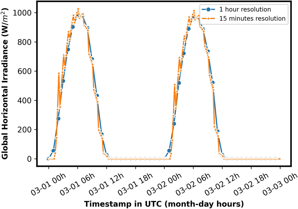
". Figure
3
shows the ECMWF forecast in its original three hourly resolution and after it is interpolated to the 15 min resolution. Similarly, the NWP output GHI from NCMRWF is also interpolated to 15 min from its original hourly resolution. The interpolated ECMWF-based GHI prediction exhibits an average bias of + 0.46% (over-estimation) against GHI measured at the PV plant over the validation period from 17.12.2018 to 23.10.2019. The interpolated GHI from NCMRWF shows a bias of + 1.71% (over-estimation). In [
4
], the nMBE in the forecast for single sites across North America and Europe over individual days ranged from − 1% to + 10%. In [
61
], the authors validated the GHI forecasts from multiple NWP models against ground measurements from stations in Southern Germany, Switzerland, Austria and Southern Spain for one year. They calculated the average bias to be between − 2.9% and + 5.9% across the sites.
Fig. 3
Interpolation of hourly GHI to 15-min resolution
Bias correction
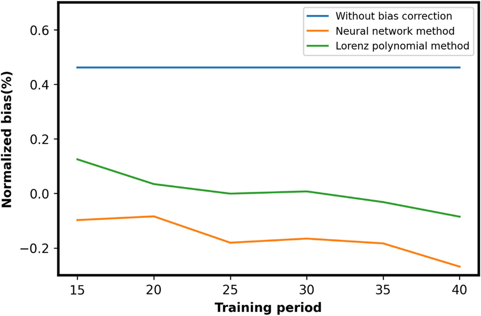
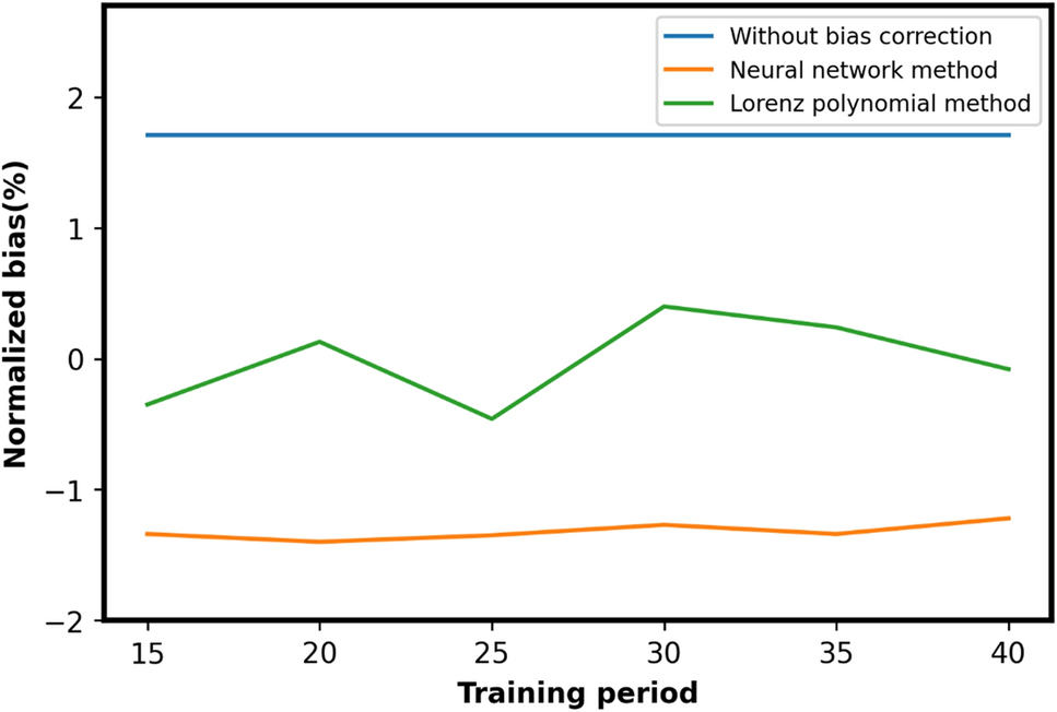
Two bias correction techniques—(i) polynomial function and (ii) NN-based bias correction methods, are validated on a sliding window basis against the ground-measured GHI from the PV plant for the period 17th December 2018 to 23rd October 2019. Ground measured GHI datasets from both the PV plant and the nearest SRRA station is used for training the two bias correction algorithms. The sliding window is varied from 15 to 40 days in 5-day steps to determine the optimum number of training days for the bias correction algorithms. The variation in bias with the change in the number of days of training in the sliding window is shown in Figs.
4
and
5
for ECMWF and NCMRWF, respectively. To select a bias correction technique for the model chain, the maximum reduction in bias with the minimum number of training days is used as a criterion. The Lorenz polynomial method reduces the bias in ECMWF predicted GHI to − 0.001% with 25 days of training. The bias in NCMRWF predicted GHI is reduced to − 0.08% with 20 days of training. After the NN-based correction, the bias lies between 0 and − 0.2% and − 1 and − 2% for ECMWF and NCMRWF respectively. Consequently, the Lorenz polynomial method is used for bias correction in the model chain. With the NN method, a negative bias is observed for all sets of training days. In [
61
], the authors performed bias correction of ECMWF predicted GHI for a period of one year. The corrected GHI predictions showed an average bias of − 0.2% against ground measurements from 87 stations distributed across north-eastern Germany.
Fig. 4
The variation of normalized bias in ECMWF output GHI with the increasing number of training days for the two bias correction methods
Fig. 5
The variation of normalized bias in NCMRWF output GHI with the increasing number of training days for the two bias correction methods
Tilt conversion
The diffuse fraction model by Chandrasekaran and Kumar” and the diffuse sky model by “Klucher” are combined in the forecasting chain for the conversion from GHI to GTI due to their suitability for Indian solar climatology (see Sect. "
Irradiance transposition
"). The PV module tilt varies seasonally at each of the five blocks. Furthermore, each block follows its own independent tilt variation schedule, and the entire manual tilt change procedure requires multiple days in each case. During the tilt changing, the PV modules in each block can have two different types of tilt values. Approximate information on tilt variation schedule was obtained from a site survey.
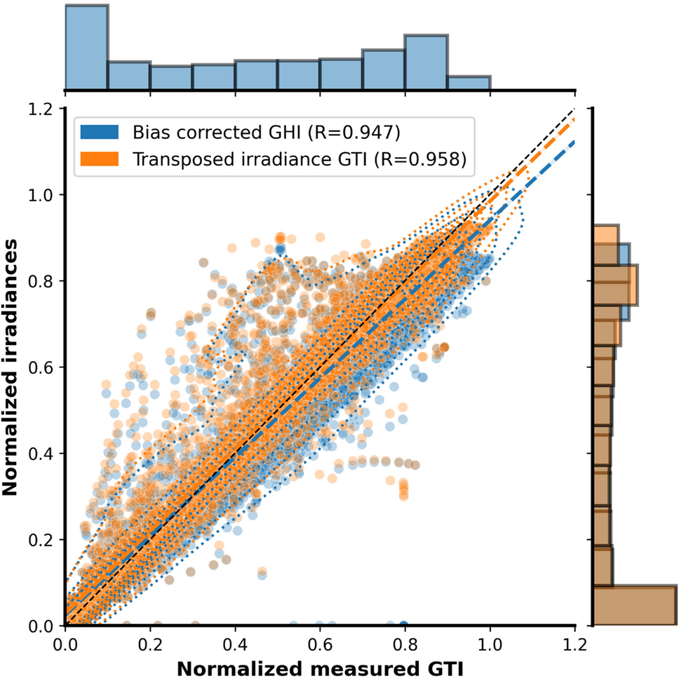
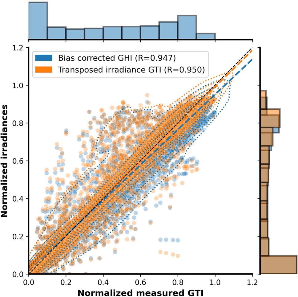
Two forecasted GTI datasets are obtained by transposing the bias-corrected GHI forecasts from the ECMWF and NCMRWF using the tilt angles from Table
1
. The forecasted GTI and forecasted GHI for the period 6th February 2019 to 6th June 2019 are plotted against the measured GTI t from a block, as shown in Figs.
6
and
7
. It can be seen that the forecasted GTI obtained by transposing GHI shows a better correlation to the measured GTI at uncertain tilt angles than the forecasted GHI. The benefit of the irradiance transposition model can be particularly observed in high-irradiance situations. [
7
] tested the performance of PV power output modeling under different scenarios—where the module tilt information is available and where it is not. By analyzing the accuracy of simulated power against measurements, it was observed that assuming a value of tilt could be better than using the GHI directly in the case of irradiance transposition with an unknown module tilt. It was also found beneficial to reduce the module tilt by 5° to 10° from its actual value. However, analyzing the final AC power accuracy has caveats as this also incorporates errors due to inaccuracies in PV module and inverter performance modeling. It can be observed from Figs.
6
and
7
that the highest utility of GHI transposition over using raw GHI is observed during periods of high irradiance, i.e., clear sky period. The benefit of using even approximate module tilt values for irradiance transposition is shown here. Especially for situations where the module tilt is changed manually on a seasonal basis, with every readjustment cycle lasting multiple days.
Fig. 6
Comparison of bias corrected ECMWF output GHI and its transposition against measured GTI
Fig. 7
Comparison of bias corrected NCMRWF output GHI and its transposition against measured GTI
DC power model
Virtual DC power data
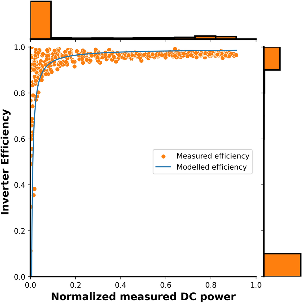
Due to the complete lack of DC measurements and block-wise AC power output data from the PV park, a synthetic or virtual DC power dataset is back-calculated from the aggregated AC power output of the entire PV park. The inverter efficiency curve from a nearby PV plant with a similar rated capacity is derived and used for this purpose, as shown in Fig.
8
. The inverter efficiency curve is obtained by training the voltage-independent Schmidt and Sauer model with actual DC and AC power output measurements from the nearby site. This efficiency curve is used to produce an aggregated virtual DC power dataset from the available aggregated AC power dataset of the PV park under analysis. [
62
] showed that the efficiency curves of grid-connected inverters vary depending on the optimization approach used. A low self-consumption strategy leads to high efficiency at small partial loads while compromising the performance at the higher end of the curve. A small input power level strategy leads to a good performance at the higher end of the curve but reduces the efficiency at small partial loads.
Fig. 8
Inverter efficiency curve estimated from a nearby PV site using Schmidt and Sauer model
PV model coefficients
The coefficients of the Huld and Beyer models are obtained by curve fitting Eqs.
13
and
16
with Virtual DC power data, GTI measurement and module temperature measurement for the period 7th November 2018 to 15th April 2019. The Beyer model additionally requires the PV module efficiency at
ηSTC
(Eq.
16
). An efficiency of 15% is assumed here as the PV modules are predominantly polycrystalline with a minor share of monocrystalline and thin film modules.
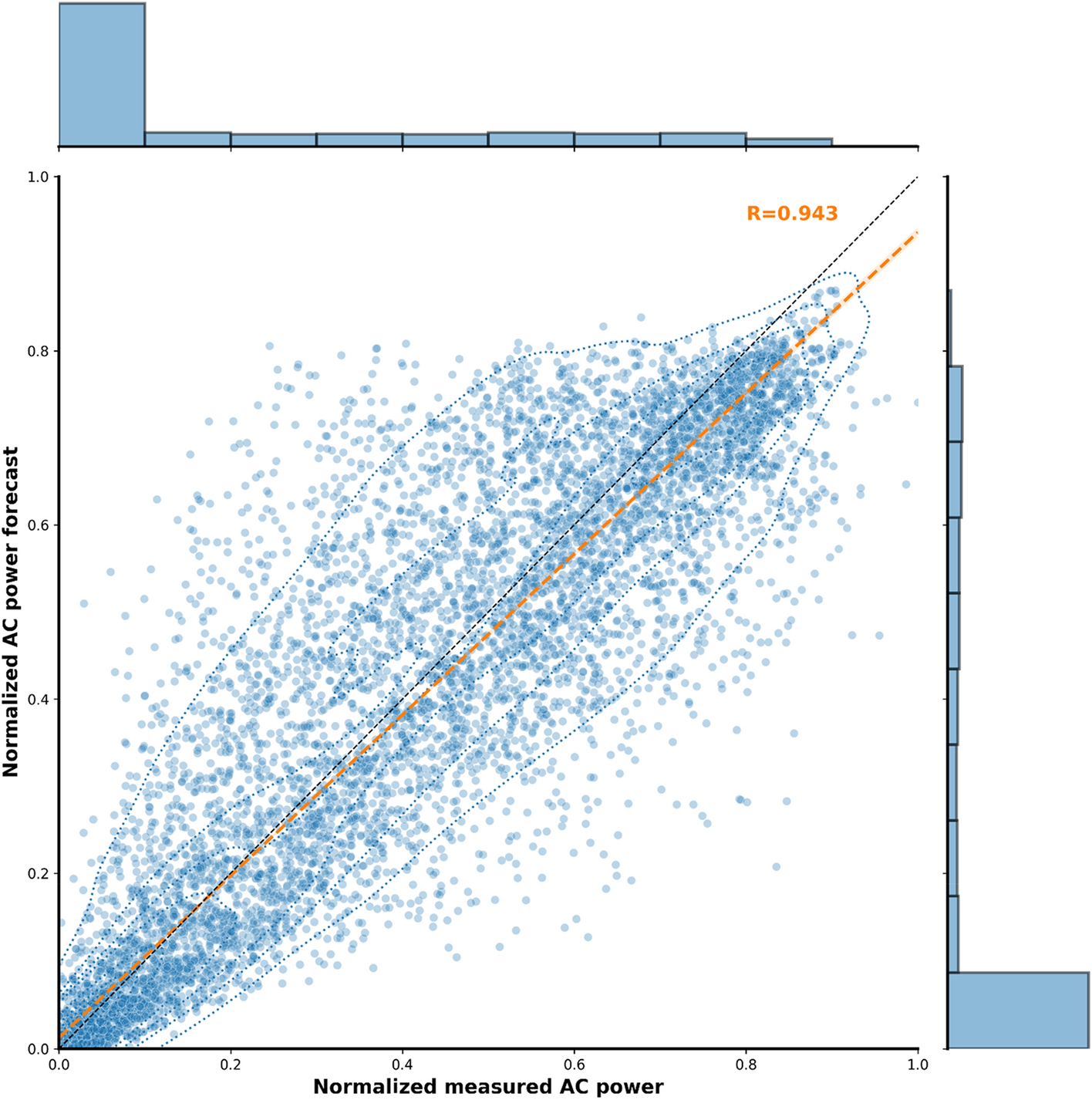
AC power predictions
The AC power predictions are calculated from the ECMWF and NCMRWF predicted GHI with the entire forecast model chain (see Fig.
1
) for the validation period of 16th April 2019 to 23rd October 2019. The Ross parameter
k
in Eq.
17
is set to 0.03 °C m
2
W
−1
based on a pre-study. With two NWP models and two GTI to DC conversion models, four forecasted AC power datasets are obtained. The error observed for these four datasets of AC power forecasts is shown in Table
2
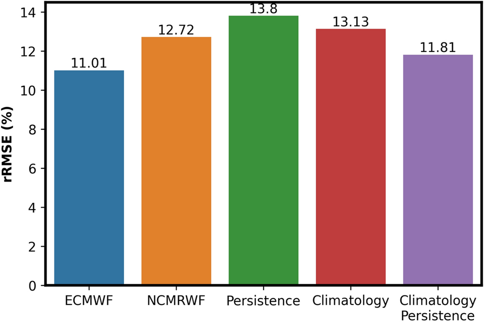
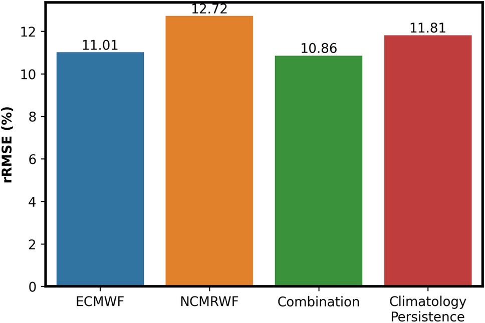
. No significant difference could be observed between the performances of Huld and Beyer models. However, as the Huld model performs marginally better, it is used in the final forecast model chain. Forecasts derived from the ECMWF and NCMRWF datasets outperform climatology and persistence, as shown in Fig.
9
. However, the NCMRWF derived forecast shows higher rRMSE than the convex combination of climatology and persistence (as defined in [
50
] and [
51
]). Figures
10
and
11
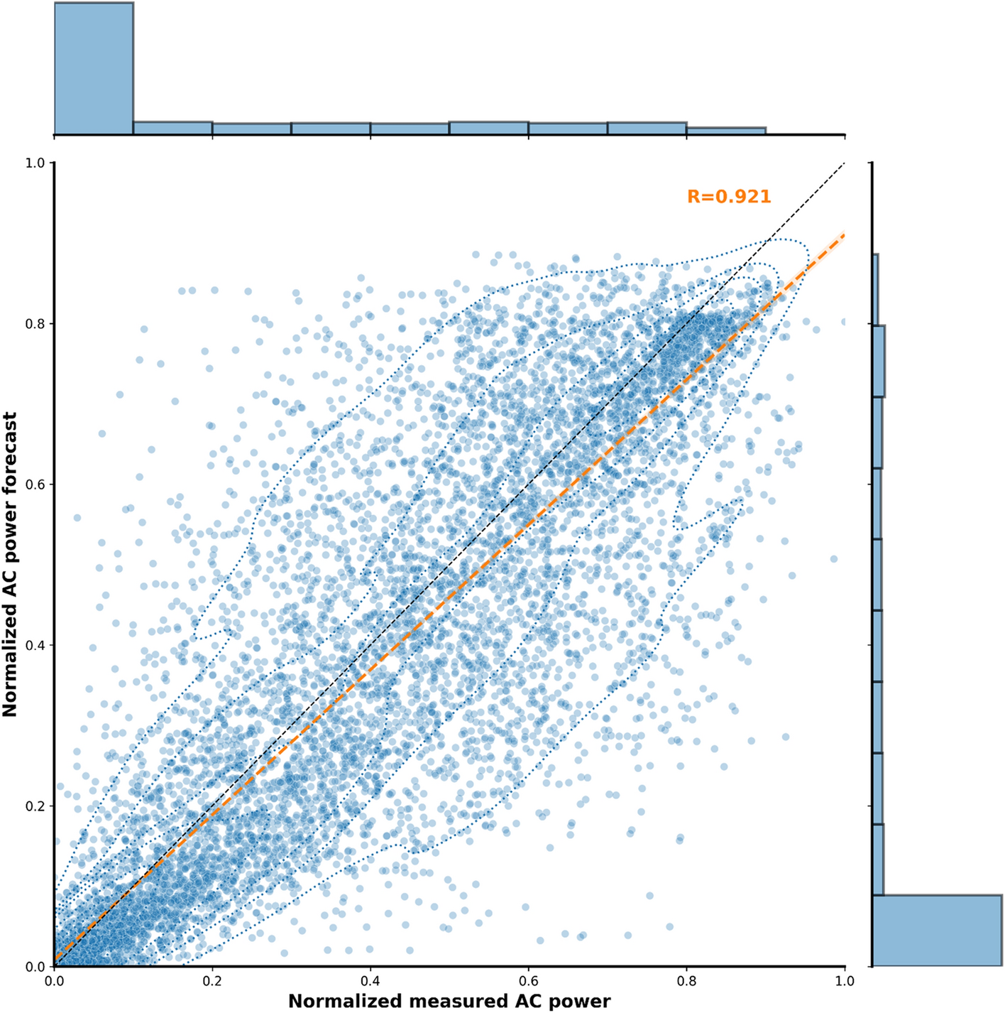
also show that NCMRWF derived forecasts show lower correlation than ECMWF. [
11
] evaluated the accuracy of their forecasting model chain against PV power measurements from China for eight exemplary days and found the nRMSE to vary between 8 and 19%. [
49
] found that the nRMSE of their model chain varied from 8.21% at 1 h ahead to 13.84% at 48 h ahead on an average for one year of PV power measurements from a site in Hungary.
Table 2
nRMSE of AC power forecasts
NWP data
Huld model (%)
Beyer model (%)
ECMWF
11.01
11.03
NCMRWF
12.72
12.76
Fig. 9
Comparison of the AC power forecasts obtained from ECMWF and NCMRWF with persistence, climatology and the convex combination of persistence and climatology
Fig. 10
AC power forecast derived from the ECMWF data
Fig. 11
AC power forecast derived from the NCMRWF data
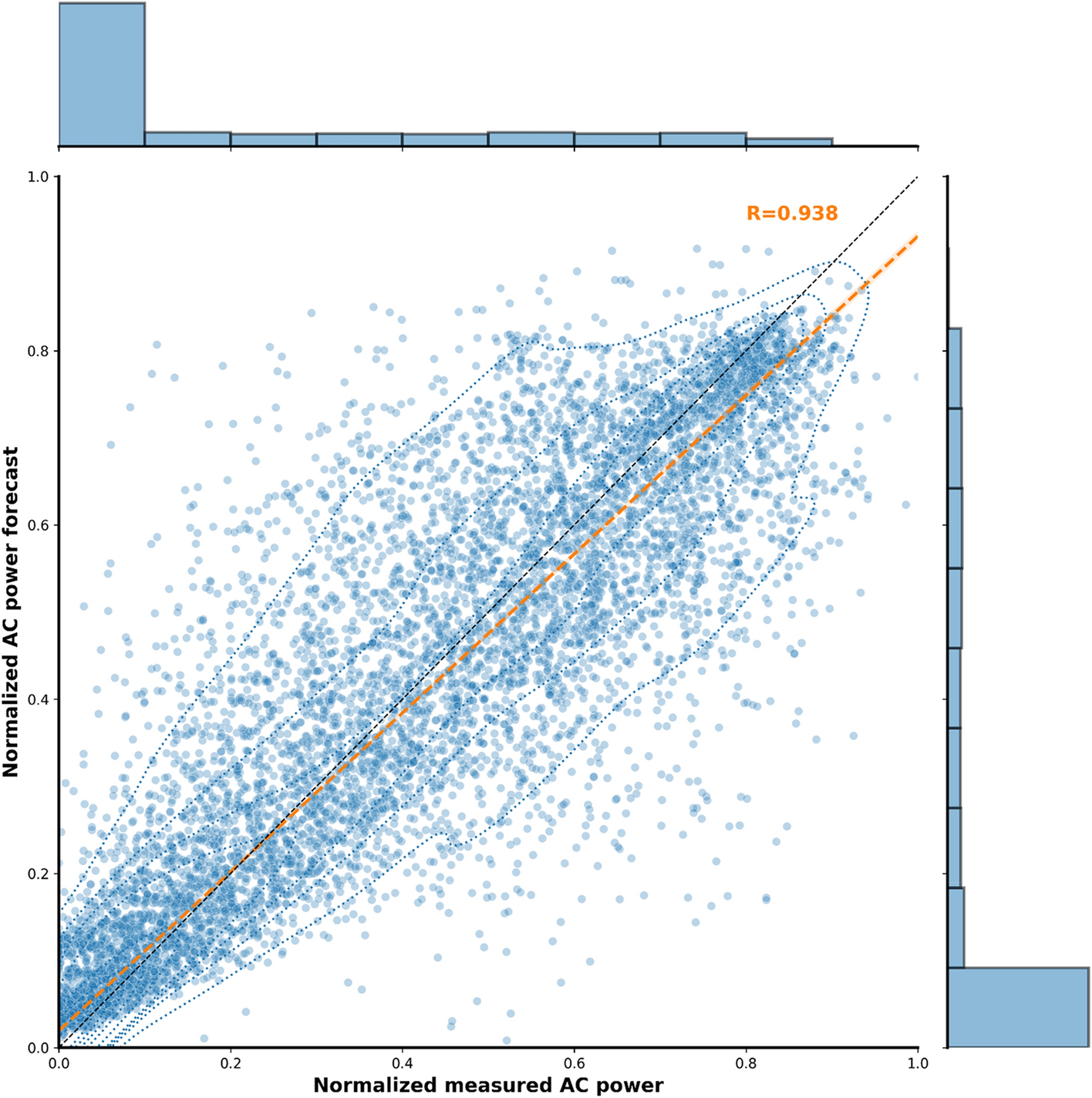
Combination of power forecasts based on the two NWP sources
For the final combined AC power prediction, the coefficients of the combination equation are trained on 15 days sliding window basis. The accuracy of the combined AC power forecast is validated for the period 1st May 2019 to 23rd October 2019. Although the NCMRWF derived forecast shows higher rRMSE than the convex combination of climatology and persistence, the final combination of ECMWF and NCMRWF derived forecasts shows the best performance, as shown in Fig.
12
. From Figs.
10
,
11
,
12
and
13
, it can be observed that there is always an underestimation of AC power for periods of higher generation that correspond to high solar elevation angles. For the periods of lower generation, an overestimation in the forecast can be observed. [
49
] showed that combination of AC power forecasts leads to a considerable improvement in accuracy at all times of the day except the early morning.
Fig. 12
Comparison of the AC power forecasts obtained from ECMWF and NCMRWF with persistence, climatology and the convex combination of persistence and climatology
Fig. 13
Combination of the AC power forecasts derived from ECMWF and NCMRWF
Conclusion
In this study, an NWP-based day ahead solar PV power forecast model chain has been developed, and each of its model component benchmarked against measurements from a 250 MWp PV park located in Southern India. Without any post-processing, the GHI output from both the ECMWF and NCMRWF models overestimated the GHI compared to the ground measurements. The Lorenz polynomial method outperformed the one hidden layer with four nodes NN architecture based bias correction method with both the NWP datasets for the PV Park site. The NN-based method also showed a consistent under-estimation of GHI with both the NWP data-sets. [
7
] opined that an assumed tilt angle may be better than using the GHI directly in situations with an unknown tilt angle. The usefulness of irradiance transposition even in situations with uncertain seasonal tilt information was established by the fact that the forecasted GTI dataset showed a better correlation with the measured GTI at uncertain tilt than the forecasted GHI with measured GTI. [
7
] did not analyze the scenario in which the AC power output dataset is available while the DC power is not. In this study, it was possible to back-calculate an aggregated virtual DC power dataset from the available aggregated AC power measurements by using a voltage-independent inverter efficiency curve derived from another nearby PV site with a similar PV capacity rating. This virtual DC power dataset was used in training the Beyer and Huld PV efficiency models. The Huld model performed only marginally better than the Beyer model and was therefore used in the final forecast model chain.. The ECMWF and NCMRWF derived forecasts outperformed both climatology and persistence. However, the NCMRWF derived forecast showed higher error than the convex combination of climatology and persistence. Nevertheless, the linear combination of the AC power forecasts derived from the ECMWF and NCMRWF datasets showed the best accuracy and outperformed the convex combination of climatology and persistence. This possibly points to the fact that the underlying atmospheric effects are modeled differently in the two NWP models, and a combination of both therefore leads to more information about the atmospheric condition. However, the global NWP models are inherently limited by their low resolution (25 km) and assume the same cloud situation or irradiance over a large area. To summarize, we demonstrated that it is possible to produce reliable day-ahead PV power forecasts, derived from numerical weather data, for the Indian subcontinent even in situations where the PV tilt information and the inverter DC measurements are lacking. Furthermore, we compared our result against a standard reference—the convex combination of persistence and climatology. Each individual step of the forecast model chain has been optimized to provide a benchmark of the expected day-ahead solar PV power forecast accuracy. As the deviation of the actual power feed-in from the forecast is penalized beyond a deviation threshold, the accuracy metrics provide solar PV plant operators information about the financial risks involved. Furthermore, as the global NWP model grid size is large (25 kms) and as there are other large solar PV parks located in the surrounding, this also gives the grid operators an idea about the expected deviation of GW scale solar PV feed-in from its day-ahead schedule. This will allow them to procure the necessary reserves in advance. The limitations in this study include:
Interpolation from 3 h or 1 h to 15 min assuming a constant clear sky index. This is not a realistic assumption, but could be improved by using a machine learning based classification.
The model chain assumes a constant tilt for the entire PV park, which is not true. Although assuming a single tilt provides better results than using GHI directly, this could be further improved upon
Although there are different kinds of PV modules connected to multiple inverters, in this study all the PV modules together and the inverters were lumped together. All properties were calculated at the aggregate level, which is not realistic. A more detailed representation of the PV park could be developed.
Global NWP models with a low spatial resolution (25 kms × 25 kms) were used in this study, whereas the solar PV park has a dimension of 3 kms × 3 kms. Regional models with higher spatial resolution will be tested in the future.
The combined AC forecast over-estimated the power production during periods with lower generation. This may be due to the inappropriate modeling of the atmospheric turbidity and scattering at low solar elevation angles. Clear sky models that incorporate near real time aerosol information could be explored for this purpose. At higher generation levels, the forecasts under-estimate the AC power. Further analysis is necessary to determine whether this under-estimation is due to the inability of NWP models to resolve clouds at the coarse resolution and the consequent averaging effect.
Acknowledgements
The authors thank the operator of the solar farm, who supported our work with historic and real-time data, the Indian Meteorological Department, who supported us with NCMRWF datasets, and GIZ GmbH, who financed a major part of the work presented. This work was carried out during 2017–2019 under the Green Energy Corridors project of the Indo-German Energy Programme. The authors declare that they have no conflict of interest.
Publisher's Note
Springer Nature remains neutral with regard to jurisdictional claims in published maps and institutional affiliations.
References
Unknown ()
Unknown ()
Unknown ()
Perez et al. (2013) Comparison of numerical weather prediction solar irradiance forecasts in the US, Canada and Europe (pp. 305-326) 10.1016/j.solener.2013.05.005
Inman et al. (2013) Solar forecasting methods for renewable energy integration (pp. 535-576) 10.1016/j.pecs.2013.06.002
Wan et al. (2015) Photovoltaic and solar power forecasting for smart grid management 1(4) (pp. 38-46) 10.17775/CSEEJPES.2015.00046
Mayer (2021) Influence of design data availability on the accuracy of physical photovoltaic power forecasts (pp. 532-540) 10.1016/j.solener.2021.09.044
Leva et al. (2017) Analysis and validation of 24 hours ahead neural network forecasting of photovoltaic output power (pp. 88-100) 10.1016/j.matcom.2015.05.010
Unknown ()
Wolff et al. (2016) Comparing support vector regression for PV power forecasting to a physical modeling approach using measurement, numerical weather prediction, and cloud motion data (pp. 197-208) 10.1016/j.solener.2016.05.051
Cui et al. (2019) Evaluating combination models of solar irradiance on inclined surfaces and forecasting photovoltaic power generation (pp. 123-130) 10.1049/iet-stg.2018.0110
Mayer and Gyula (2021) Extensive comparison of physical models for photovoltaic power forecasting10.1016/j.apenergy.2020.116239
Unknown ()
Huang and Thatcher (2017) Assessing the value of simulated regional weather variability in solar forecasting using numerical weather prediction (pp. 529-539) 10.1016/j.solener.2017.01.058
Lorenz et al. (2009) Irradiance forecasting for the power prediction of grid-connected photovoltaic systems (pp. 2-10) 10.1109/JSTARS.2009.2020300
Joshi et al. (2019) Evaluation of solar irradiance forecasting skills of the Australian Bureau of Meteorology’s ACCESS models (pp. 386-402) 10.1016/j.solener.2019.06.007
Unknown ()
Suksamosorn et al. (2021) Post-processing of NWP forecasts using kalman filtering with operational constraints for day-ahead solar power forecasting in Thailand (pp. 105409-105423) 10.1109/ACCESS.2021.3099481
Yang (2019) On post-processing day-ahead NWP forecasts using Kalman filtering (pp. 179-181) 10.1016/j.solener.2019.02.044
Lauret et al. (2014) A neural network post-processing approach to improving NWP solar radiation forecasts (pp. 1044-1052) 10.1016/j.egypro.2014.10.089
Lauret et al. (2016) Solar forecasting in a challenging insular context10.3390/atmos7020018
Pereira et al. (2019) Development of an ANN based corrective algorithm for the operational ECMWF global horizontal irradiation forecasts (pp. 387-405) 10.1016/j.solener.2019.04.070
Watanabe et al. (2021) Post-processing correction method for surface solar irradiance forecast data from the numerical weather model using geostationary satellite observation data (pp. 202-216) 10.1016/j.solener.2021.05.055
Tschopp et al. (2022) Measurement and modeling of diffuse irradiance masking on tilted planes for solar engineering applications (pp. 365-378) 10.1016/j.solener.2021.10.083
Chandrasekaran and Kumar (1994) Hourly diffuse fraction correlation at a tropical location (pp. 505-510) 10.1016/0038-092X(94)90130-T
Skartveit et al. (1998) An hourly diffuse fraction model with correction for variability and surface albedo 63(3) (pp. 173-183) 10.1016/S0038-092X(98)00067-X
Paulescu and Blaga (2019) A simple and reliable empirical model with two predictors for estimating 1-minute diffuse fraction (pp. 75-84) 10.1016/j.solener.2019.01.029
Furlan et al. (2012) The role of clouds in improving the regression model for hourly values of diffuse solar radiation (pp. 240-254) 10.1016/j.apenergy.2011.10.032
Ridley et al. (2010) Modelling of diffuse solar fraction with multiple predictors 35(2) (pp. 478-483) 10.1016/j.renene.2009.07.018
Batzelis (2017) Simple PV performance equations theoretically well founded on the single-diode model (pp. 1400-1409) 10.1109/JPHOTOV.2017.2711431
Yaqoob et al. (2021) Comparative study with practical validation of photovoltaic monocrystalline module for single and double diode models10.1038/s41598-021-98593-6
Unknown ()
Deotti et al. (2021) Empirical models applied to distributed energy resources-an analysis in the light of regulatory aspects 14(2) 10.3390/en14020326
Huld et al. (2011) A power-rating model for crystalline silicon PV modules (pp. 3359-3369) 10.1016/j.solmat.2011.07.026
Soler-Castillo et al. (2021) Modelling of the efficiency of the photovoltaic modules: grid-connected plants to the Cuban national electrical system (pp. 150-157) 10.1016/j.solener.2021.05.052
Padmavathi and Arul (2013) Performance analysis of a 3 MWp grid connected solar photovoltaic power plant in India (pp. 615-625) 10.1016/j.esd.2013.09.002
Santiago et al. (2018) Modeling of photovoltaic cell temperature losses: a review and a practice case in South Spain (pp. 70-89) 10.1016/j.rser.2018.03.054
Skoplaki et al. (2008) A simple correlation for the operating temperature of photovoltaic modules of arbitrary mounting (pp. 1393-1402) 10.1016/j.solmat.2008.05.016
Roumpakias and Stamatelos (2019) Performance analysis of a grid-connected photovoltaic park after 6 years of operation (pp. 368-378) 10.1016/j.renene.2019.04.014
Unknown ()
King et al. (2004) Photovoltaic array performance model10.2172/919131
Unknown ()
Unknown ()
Schmidt and Sauer (1996) Wechselrichter-Wirkungsgrade (pp. 43-47)
Yang and Meer (2021) Post-processing in solar forecasting: ten overarching thinking tools10.1016/j.rser.2021.110735
Böök and Lindfors (2020) Site-specific adjustment of a NWP-based photovoltaic production forecast 211(15) (pp. 779-788) 10.1016/j.solener.2020.10.024
Unknown ()
Yang (2019) Standard of reference in operational day-ahead deterministic solar forecasting10.1063/1.5114985
Yang (2019) Making reference solar forecasts with climatology, persistence, and their optimal convex combination (pp. 981-985) 10.1016/j.solener.2019.10.006
Kumar et al. (2014) Field experiences with the operation of solar radiation resource assessment stations in India10.1016/j.egypro.2014.03.249
Schwandt et al. (2014) Quality check procedures and statistics for the Indian SRRA solar radiation measurement network (pp. 1227-1236) 10.1016/j.egypro.2014.10.112
Ineichen and Perez (2002) A new airmass independent formulation for the linke turbidity coefficient (pp. 151-157) 10.1016/S0038-092X(02)00045-2
Rincón et al. (2018) Bias correction of global irradiance modelled with weather and research forecasting model over Paraguay (pp. 201-211) 10.1016/j.solener.2018.05.061
Liu and Jordan (1963) The long-term average performance of flat-plate solar-energy collectors: with design data for the U.S., it’s outlying possessions and Canada 7(2) (pp. 53-74) 10.1016/0038-092X(63)90006-9
Temps and Coulson (1977) Solar radiation incident upon slopes of different orientations 19(2) (pp. 179-184) 10.1016/0038-092X(77)90056-1
Faiman (2008) Assessing the outdoor operating temperature of photovoltaic modules (pp. 307-315) 10.1002/pip.813
Unknown ()
Unknown ()
Notton et al. (2010) Optimal sizing of a grid-connected PV system for various PV module technologies and inclinations, inverter efficiency characteristics and locations 35(2) (pp. 541-554) 10.1016/j.renene.2009.07.013