Geometrical nonlinearities and shape effects in electromechanical models of piezoelectric bridge structures

Introduction

The application of nonlinear mechanical structures in inertial energy harvesting using piezoelectric transduction is a growing field of research motivated by the potential advantages over linear resonator systems in terms of bandwidth, durability and amplitude [ ¹ , ² , ³ , ⁴ – ⁵ ]. In addition, manifestly nonlinear modes of operation have been suggested to target excitation regimes where linear systems typically produce insufficient power [ ¹ , ⁶ , ⁷ – ⁸ ]. Conversely, microelectromechanical (MEMS) piezoelectric actuators and switches are characterized by fast response and high bandwidth [ ⁹ ] and able to produce large amplitude actuation. Accurate operation in the large deflection regime requires accounting for nonlinear effects both in terms of the displacement and the voltage applied to produce it [ ¹⁰ , ¹¹ ].

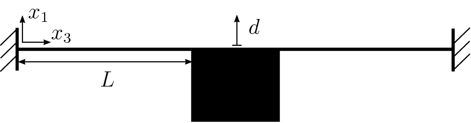
A common structure in applications, which features mechanical nonlinearities, is the doubly clamped bridge with a central proof-mass, as illustrated in Fig.  ¹ . At infinitesimal deflections d of the proof-mass, the deformation of the beams is described by the Euler-Bernoulli theory of bending strain and the restoring force is linear in d . However, at finite deflections d , the boundary conditions and symmetry of the problem induce stretching strain in the beams, corresponding to nonlinear contributions to the restoring force. At deflections d which are large compared to the thickness of the beams, nonlinear effects must be accounted for to accurately describe the system [ ¹ , ⁵ ]. In addition, the shape of the beams, i.e., the functional coordinate dependence of the displacement field, depends on both the proof-mass displacement d and the voltage v which must be accounted for.

Fig. 1

The purpose of the present paper is the derivation and validation of a theoretical model describing the shape of the beams in the piezoelectric bridge structure as a function of the displacement d and voltage v , as well as a lumped model for the piezoelectric bridge structure, that is a system of differential equations governing the displacement d and voltage v . Such a theoretical model provides a way to understand how shape effects enter into both the static and dynamical properties of the system and is essential for accurately designing structures for various applications in the domain of large deflections and voltages.

A variational approach was used in [ ¹² ] to compute large d corrections to the nominal shape function (valid at infinitesimal d ) in a purely mechanical bridge structure. In the present paper, we extend the analysis to a piezoelectric bridge structure by including electromechanical effects in the description of the system. Consequently, the shape function acquires a dependence on the electric voltage v across the piezoelectric layer in addition to the deflection d . We construct a model for the electromechanical bridge based on a power series Ansatz for the shape function and perform a variational analysis to derive conditions corresponding to the minimization of the Gibbs enthalpy. We also compute explicitly the lowest order corrections to the nominal shape function and validate the resulting model using finite element model (FEM) simulations. Finally, we derive the equations of motion for the model including the lowest order correction by incorporating the electromechanical shape effects, and discuss their impact on the dynamics of the system.

The variational approach results in an improved electromechanical model of piezoelectric bridge structures accounting for electromechanical shape effects, extending the work by Gafforelli et al. [ ⁶ ]. The importance of including the shape effects in order to accurately model the operation of bridge type harvesters, sensors and actuators in realistic applications where nonlinear effects are significant is demonstrated.

In addition to clearly displaying the the functional relationships between design parameters and nonlinear effects in the system, the lumped model offers significant advantages over FEM simulations in terms of computational cost and possibilities to explore parameter space. In particular, this is true for the simulation of system dynamics where the nonlinearities require computationally intensive time-dependent FEM simulations where the time step required for accuracy is typically several orders of magnitude smaller than the time scale of the dynamics of the system and transient phenomena.

Lumped models of the bridge structure (as well as other common structures appearing in MEMS applications) have been derived before and have proven extremely useful [ ⁵ , ⁶ , ¹³ ]. In [ ⁶ ], a Rayleigh-Ritz method was employed to derive a nonlinear model of the piezoelectric bridge based on a time-dependent rescaling of the Euler-Bernoulli displacement profile valid a infinitesimal amplitudes. A similar approach was previously used to derive a nonlinear model of microcantilever actuators [ ¹⁴ ] and its extension to a nonlinear modal analysis was considered in [ ¹⁵ , ¹⁶ ]. Furthermore, the approach utilized in the derivation of our model has been successfully applied on numerous occasions in the form of a Galerkin method used to model geometrical nonlinearities in the context of efficient full spatio-temporal numerical simulations of MEMS structures [ ¹⁷ , ¹⁸ ]. However, to the best of our knowledge, the model presented in the present paper is the first lumped model of the piezoelectric bridge system accounting for geometrical nonlinearities and incorporating their effect on the shape of the bridge.

Electromechanical model

In this section, we consider a nonlinear electromechanical model of a piezoelectric bimorph operating in the e31 mode, and the boundary conditions associated with a doubly clamped bridge structure. At large deflections d , the mechanical strain according to Green-Lagrange is given as the sum of a bending strain and a stretching strain

Boundary conditions

The mechanical boundary conditions for a single beam are

w1x3=0=0,w1x3=L=d

∂w1∂x3x3=0=0,∂w1∂x3x3=L=0.

In addition, we assume that the w1 displacement field is independent of both the x1 and the x2 coordinates. In this situation, the symmetry of the problem implies that the function w1 is antisymmetric with respect to x3=L/2 , which imposes additional constraints on the derivatives of the displacement w1 according to

∂nw1∂x3nx3=L/2=0,n∈2N1,

where N1 is the set of all positive integers ² . We will discuss the properties of the structure required for the assumption ∂w1/x2=0 to be valid in more detail below.

Furthermore, symmetry of the bridge configuration preventing displacement of the proof mass in the x3 -direction imposes zero x3 -displacement conditions at x3=0 and x3=L implying that the deformation w1 is associated with a change in length of the harvester and that the in-plane displacement field w3 and its derivatives can be safely neglected.

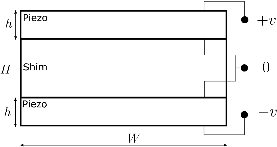
The electrical boundary conditions depend on the details of the piezoelectric layer configuration. We will consider a bimorph configuration illustrated in Fig.  ² . In order to utilize the stretching strain contribution dominating at large deflection, the polarized piezoelectric region and the corresponding electrode extend the full length of the beam. We note that using this electrode configuration, the bending strain contributions to the electromechanical energy will cancel identically.

Fig. 2

Variational analysis

The defining property of the shape function w(ξ) is that it minimizes the Gibbs enthalpy V subject to the boundary conditions. The shape function that extremizes the functional V[w] can be found as the solution to the variational equation ⁴ .

We will use a power series Ansatz for the shape function in the dimensionless length parameter ξ

In practice, we will truncate the power series at some power N , in order to simplify the problem and determine a suitable approximation for the true shape function. It should be noted that this is different from an ordinary perturbation theory expansion of a scalar quantity in terms of a small parameter, since ξ is actually a coordinate and the minimization is performed over the entire domain. However, due to symmetry, the shape function is uniquely determined by its values over the interval ξ∈[0,1/2] where higher powers of ξ are suppressed. Furthermore, the approximate strain energy V is a decreasing function of N since as we add higher powers to w(ξ) a solution with unchanged energy is obtained by simply setting all added coefficients an=0 . Therefore, in the limit N→∞ , we expect to approach the exact solution.

In the first part of this section, we will provide some general results and describe the method used to find the approximate shape function w for arbitrary N . Subsequently, we will exemplify the procedure for N=5 which represents the first correction to the trivial (in a sense to be made precise below) shape function.

N=5\documentclass[12pt]{minimal} \usepackage{amsmath} \usepackage{wasysym} \usepackage{amsfonts} \usepackage{amssymb} \usepackage{amsbsy} \usepackage{mathrsfs} \usepackage{upgreek} \setlength{\oddsidemargin}{-69pt} \begin{document}$$N=5$$\end{document} corrections

Truncating the general expressions for boundary and symmetry conditions at N=5 , we can now compute the first corrections to ( ³⁶ ). For N=5 , there is only one independent coefficient, which we take to be a5=a . The boundary conditions and the n=2 symmetry constraint allow us to express the dependent coefficients as

a2=3d-12a,a3=-2d+2a,a4=-52a.

The computation of the bending and stretching contributions Vb and Vs are straightforward, if somewhat tedious, yielding

Vb(a,d)=12d2+17a2,

Vs(a,d)=7235d4+72385ad3+6455a2d2+15005a3d+1255255a4

and

Vem(a,d)=6d25+ad35+a2630.

Inserting these expressions into the variational equation allow us to compute the parameter a as the solution to ( ³⁵ ) and the corresponding N=5 shape function and enthalpy as a function of d and v .

The purpose of computing corrections to the shape function is to obtain an improved estimate compared to the lowest order N=3 function, which we have seen describes the pure bending situation at infinitesimal displacements and applied voltages and is therefore not expected to properly account for large deformations of the doubly clamped structure or large electrical fields. In the form derived above, the variational problem depends on the electromechanical properties and the geometry of the bridge structure.

In order to obtain results which are independent of the precise properties and geometry of the structure, we introduce dimensionless quantities

α=aλ,δ=dλ,ν=μ2vλ2

where the characteristic length and voltage scales of the problem are given by

λ2=AbAs,μ2=AemAs.

We also introduce the dimensionless shape enthalpy

W=Vb(α,δ)+Vs(α,δ)+Vem(α,δ)ν,

which contains only shape-dependent terms which will contribute to the variation with respect to w . The variational condition determining the bridge shape is then finally given as

∂W∂α=4255255α3+3δ5005α2+12δ2455+ν315+27α+72δ3385+δν35=0.

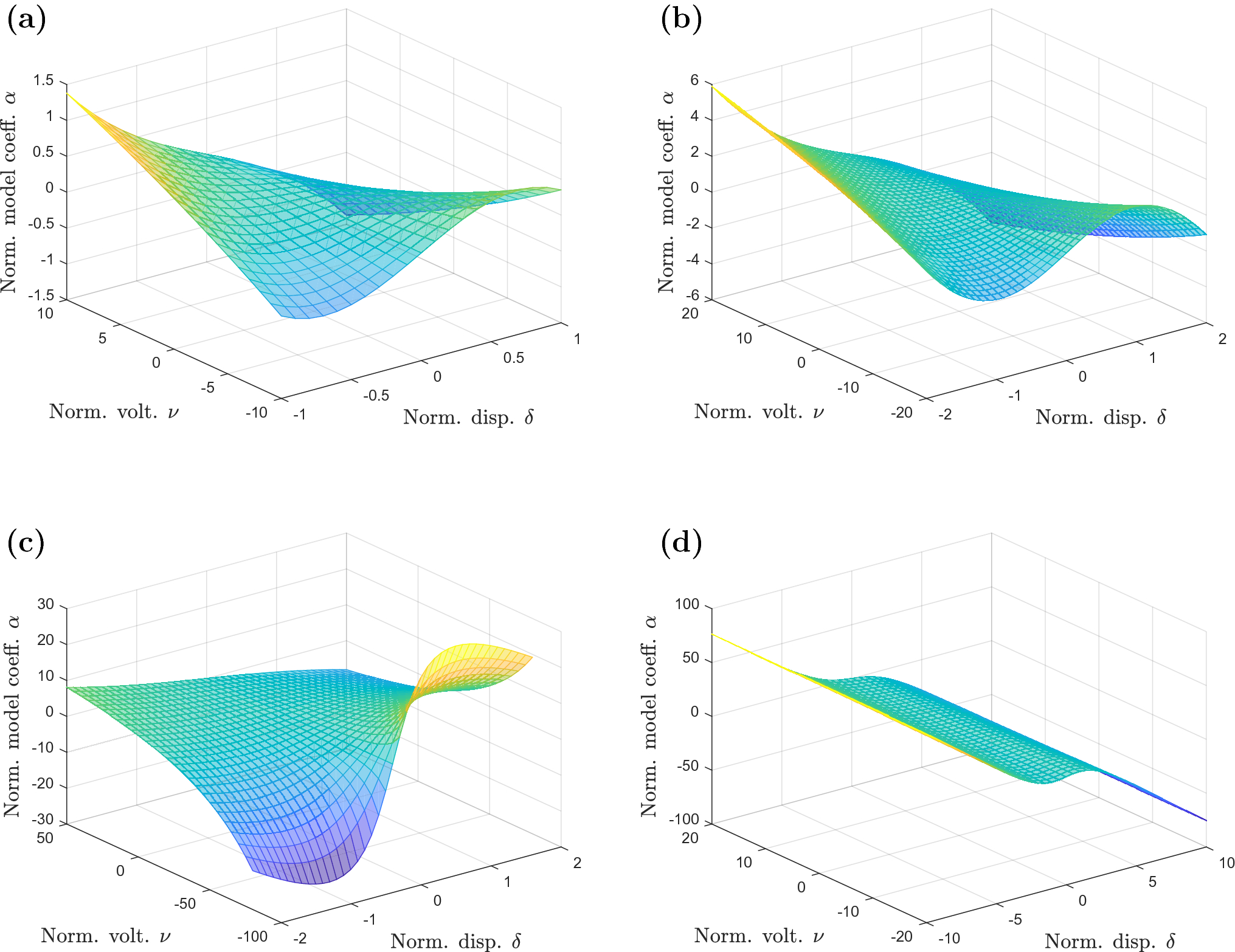
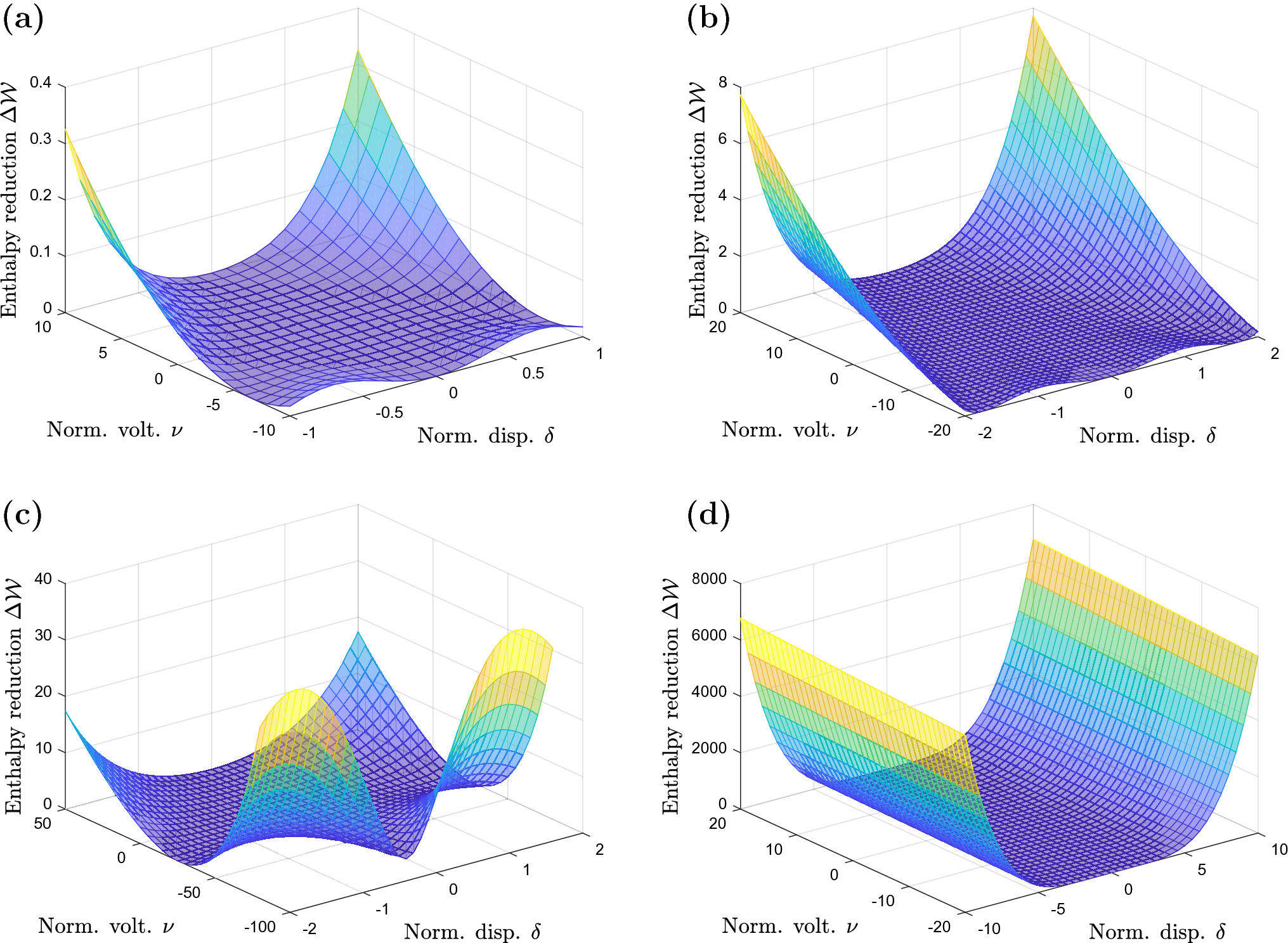
This is a cubic equation which we can solve numerically for α given the dimensionless displacement δ and voltage ν , yielding the results in Fig.  ³ for different ranges of the dimensionless displacement and voltage. We note that since the enthalpy is not manifestly positive, the relative reduction of W in the N=5 model compared to the N=3 model is not a meaningful (or even regular) measure. Therefore, the dimensionless shape enthalpy reduction is used to quantify the improvement in model accuracy in Fig. ⁴ . We note that in all cases the reduction is non-negative implying that the shape enthalpy W3 in the N=3 model is larger than the corresponding quantity W5 in the N=5 model.

Fig. 3

Fig. 4

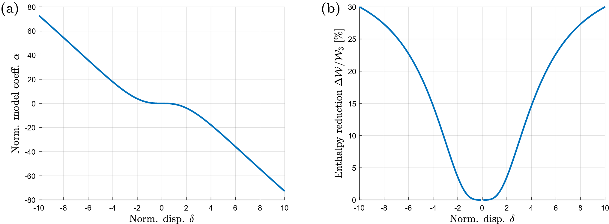
As a special case, setting ν=0 reproduces the results in the purely mechanical case [ ¹² ]. In this case, the enthalpy reduces to potential strain energy and the relative reduction becomes well-defined. The parameter α and the relative reduction in strain energy ΔW are show in Fig. ⁵ .

Fig. 5

It is straightforward to verify numerically that for the range of δ and ν considered here, the discriminant of the cubic Eq. ( ⁴⁴ ) is negative, implying that the existence of a single real root which guarantees the uniqueness of the numerical solution.

Model validation

While it is clear from the results presented in the previous section that the N=5 model provides a (substantial) improvement compared to the N=3 model, it remains to validate the variational approach in comparison with the physical systems it is meant to describe, and to quantify the improvement obtained by including the N=5 model corrections in this context. To this end, the theoretical models are evaluated for a validation model and compared to the results obtained using a large deflection FEM simulation model accounting for geometrical nonlinearities.

Validation results

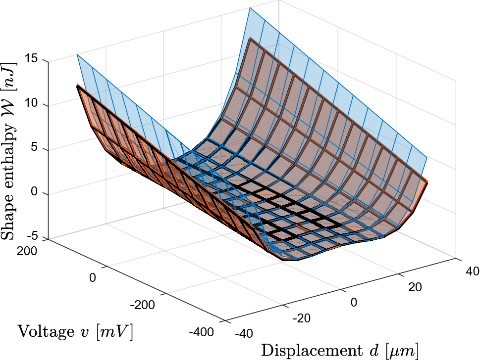
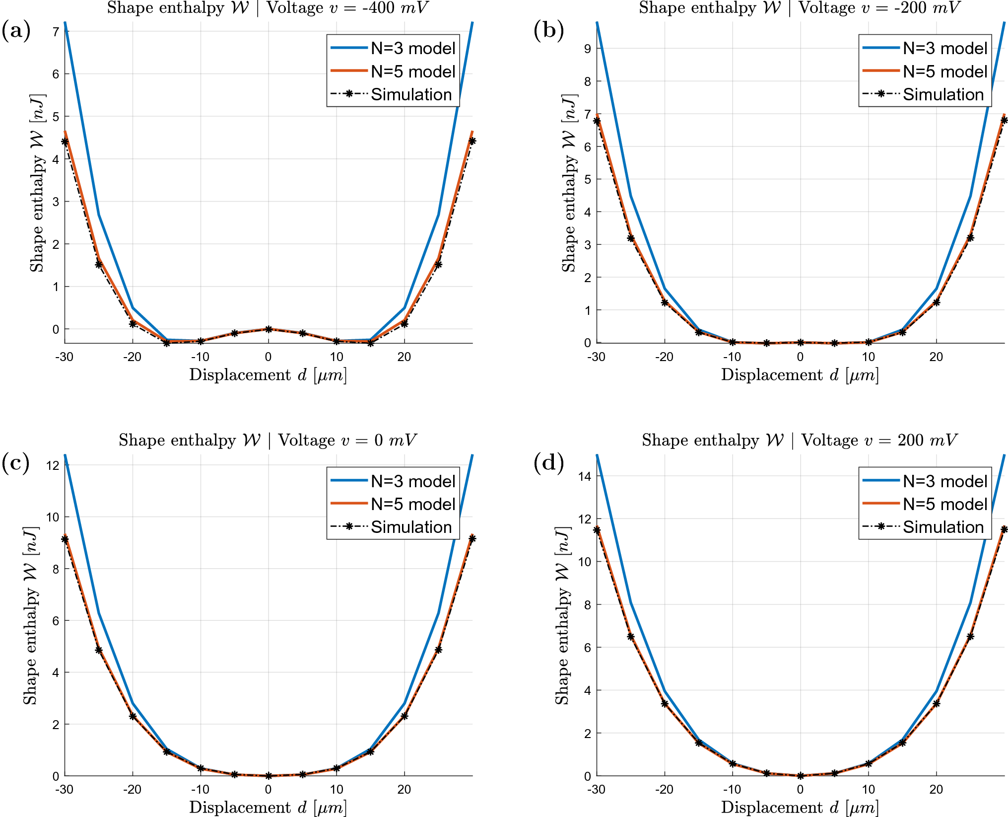
The primary quantification of the improvement obtained by accounting for the N=5 corrections is the Gibbs enthalpy. As above, we are primarily concerned with the part that depends on the shape function, that is the shape enthalpy W . For the validation ranges specified above, the shape enthalpy W is shown as a function of both d and v in Fig.  ⁶ , and as a function of d for constant voltage v in Fig.  ⁷ . It is clear from the results that the N=5 corrections compensate for essentially the entire enthalpy error caused by the incorrect assumption of the form of the shape function in the N=3 model. Furthermore, the improvement is significant in the range considered in the validation model. For example, at d=30μ m and v=200 mV, the error relative to the simulation is reduced from 30% in the N=3 model to 2% in the N=5 model.

Fig. 6

Fig. 7

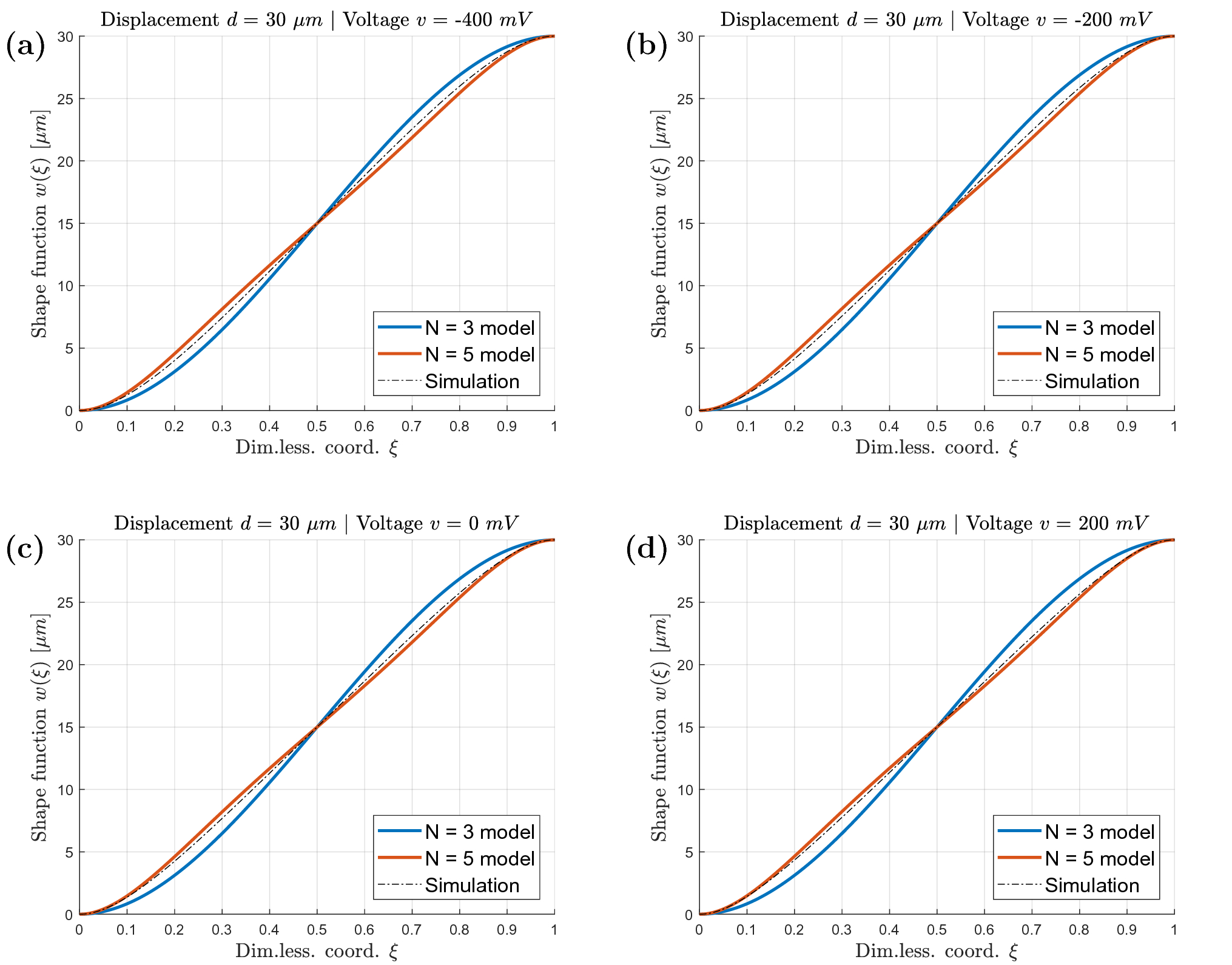
The shape function w(ξ) can also be validated using the simulation model. Figure  ⁸ shows results obtained from the theoretical models and the simulation model for proof-mass displacement d=30μ m. While it is not obvious how to quantify the improvement in terms of the shape function in a physically relevant way, the N=5 model appears to produce a better qualitative agreement with the simulated results than does the N=3 model. We also note that the FEM simulation validates the boundary conditions ( ⁵ )–( ⁷ ).

Fig. 8

System dynamics

In this section, we incorporate the shape effects considered above into the equations of motion for the electromechanical bridge system, in order to account for their influence on the dynamics of the system. To accomplish this, we use the Euler-Lagrange equations which are conveniently formulated in suitable generalized coordinates of the system. The Euler-Lagrange approach yielding equations of motion for the lumped variables are applicable since the time scale of spatial strain and voltage equilibration in the structure is typically orders of magnitude smaller than the time scale of the change of global variables in applications.

For the bridge structure, the fundamental quantity in the electrical domain is the charge q separated across the piezoelectric layer. The rate of change in q is related to the voltage v across the layer by the continuity equation in the electrical domain, the precise form of which depends on the effective external impedance between the top and bottom electrode. We will consider the case where the circuit connecting the electrodes is a simple resistive load R , which is a common choice in, e.g., the energy harvesting literature and makes it easy to consider the open and closed circuit dynamics as the limiting cases R→∞ and R→0 , but a more general terminating circuit can be considered in an analogous way. The equation of continuity is then

The dynamics of the system is governed by the Euler-Lagrange equations for the generalized coordinates {q1,q2}={d,q}

Conclusion

In this paper, we have shown how nonlinear shape effects appear in the lumped electromechanical model of a bimorph piezoelectric bridge structure. Under broadly applicable assumptions regarding the form of the Green-Lagrange strain, these effects arise from the interaction between the electromechanical constitutive model and the geometry of the structure. At finite proof-mass displacement and electrode voltage, the shape of the beams minimizing the Gibbs enthalpy is no longer the solution of Euler-Bernoulli theory, which influences the coupling between the electrical and mechanical domains.

Adding higher order terms in ξ to the Euler-Bernoulli solution, we use a variational approach to derive corrections to the shape function of any order. The lowest order N=5 corrections are parametrized by a single dimensionless model coefficient α and we derive explicitly the equilibrium equation determining α as a function of the dimensionless displacement δ and voltage ν . Numerical solution of the governing Eq. ( ⁴⁴ ) reveals an intricate nonlinear dependence of both the model coefficient and the (shape-dependent part of) the enthalpy on δ and ν . For a large range of displacements and voltages, we show that the corrections to the shape function produce a reduction in the shape enthalpy corresponding to an improved model accuracy.

Subsequently, we validate the theoretical model using large deflection FEM simulations of a bridge structure in the MEMS regime. The validation model and the simulated ranges of displacements and voltages are selected to be representative of both the energy harvesting (or sensing) and the actuation modes of operating the structure. The validation results indicate that the N=5 model represents a substantial improvement of the lowest order N=3 model. In fact, the accuracy achieved by the N=5 model in terms of the Gibbs enthalpy and shape function is expected to be sufficient for most applications.

Finally, we derive explicitly the equations of motion for the N=5 model and show how the coupling between the electromechanical properties and the geometry of the bridge structure introduces nonlinear interaction terms. The equations of motion follow directly from the Euler-Lagrange equations by inserting the expression for the N=5 Gibbs enthalpy W , which has been independently validated.

As always, there are limitations associated with the assumptions made in the derivation of the model presented here. Such limitations include the restriction to a linear constitutive relation ( ³ ) and a linear relation ( ⁹ ) between the voltage and electric field as well as ignoring any spatial electromechanical fringe effects. In addition, no estimates of the convergence of the power series approximation as N increases are provided. While the numerical validation suggests that already the N=5 model is sufficient for most applications, it is important to keep such theoretical limitations in mind, in particular when considering extending the scope of the model.

Care must also be taken extending the ranges of (dimensionless) displacement and voltage in the model. The discriminant of the third degree polynomial Eq. ( ⁴⁴ ) can become non-negative for some values of δ and ν , which corresponds to multiple real roots, and multiple local extrema of the enthalpy, which must be investigated to determine the global minimum and the corresponding shape function.

The theoretical modelling of nonlinear piezoelectric structures can be motivated as a tool to make accurate predictions of the behaviour of structures appearing in applications to sensing, energy harvesting or actuation at a fraction of the computational cost of FEM models. However, perhaps the most important aspect of the theoretical lumped model is its potential to produce a deeper understanding of the system under investigation by identifying the underlying mathematical structures. More specifically, this includes the functional dependence of the coupling constants appearing in both the static and dynamical model on the geometrical and electromechanical parameters of the system. Such an understanding is essential for a successful and systematic design process in practical applications. In conclusion, the present paper elucidates the interaction between the geometry and the electromechanical properties of a nonlinear bridge structure and shows that this interaction must be accounted for in order to obtain accurate models in several common applications of piezoelectric devices.