Flare performance modeling and set point determination using artificial neural networks

Introduction and literature survey

When utilization or conservation of waste gas streams is not practicable, flaring is environmentally preferable to venting since this tends to reduce Green House Gases, Volatile Organic Compounds (VOC), and Hazardous Air Pollutants (HAPs) emissions. This seemingly simple process is rather complicated since flare performance is affected by many parameters, most of which never remain constant. The most common among these variables are the fuel to air-/steam-assist ratios, the heating value of the fuel, jet velocity, and meteorological conditions. Flare gas emissions are primarily estimated based on a few assumptions about the volume of gas sent to the flare stack, its chemical composition, and the presumed combustion efficiency [ ¹ , ² ]. Although the USEPA states that destruction efficiency for normal industrial flaring practices is 98%, these assumptions are under scrutiny by agencies these days.

The U.S. Environmental Protection Agency (EPA) estimates there are about 500 flares in over 100 U.S. refineries but many more in chemical plants and drilling sites. The number of permits for flaring in Texas rose from just over a hundred in 2008–2000 in 2012 [ ³ , ⁴ , ⁵ – ⁶ ]. The world bank estimates that about 140 billion cubic meters of gas was flared in 2016–2017 globally, which is about 7 billion cubic meters less than 2016 [ ⁴ ]. Improper operation of an industrial flare can result in hundreds of tons of excess air toxics emissions. Air emissions may contribute to increased ground-level ozone and climate change [ ⁷ , ⁸ , ⁹ , ¹⁰ , ¹¹ , ¹² – ¹³ ]. Large sources of methane emissions from natural gas production were observed from shale gas wells. Fugitive methane emissions in the production process can counter the advantages over coal with respect to climate change [ ⁹ , ¹⁰ ]. Visible Infrared Imaging Radiometer Suite data may provide site-specific tracking of natural gas flaring to evaluate efforts to reduce and eliminate routine flaring [ ¹⁴ , ¹⁵ ]. Proper flare design considerations are required to safely dispose of the waste gases, some of which include the type of flare (gas/liquid), composition of fuel, temperature, flowrate, gas pressure and hydraulics [ ⁵ , ¹⁶ , ¹⁷ , ¹⁸ – ¹⁹ ]. In a research by Ismail et al., percentage of stoichiometric air, natural gas type, carbon mass content, impurities and combustion efficiency of the flare system impact the quantity and pattern of chemical species in combustion zone during flaring [ ⁶ ]. Incomplete combustion from flares contributes to black carbon (soot) emissions. Plume samples from 37 unique flares in the Bakken region of North Dakota in May 2014 showed no obvious relationship between methane and BC emission factors. It was observed that efficiency distribution was skewed, exhibiting log-normal behavior [ ¹³ ]. There is a need to consider skewed distributions when assessing flare impacts globally.

In the Fact Sheet for the Proposed Petroleum Refinery Sector Risk and Technology Review and New Source Performance Standards, the EPA states that the proposed new standards for flares will decrease VOC (Volatile Organic Compound) emissions from flares by 33,000 tons per year [ ²⁰ , ²¹ , ²² , ²³ , ²⁴ , ²⁵ – ²⁶ ]. It is also estimated that the total VOC emission reductions for all affected sources in this proposed rule are 52,000 tons per year. The flare portion accounts for 63% of the total reductions. There are more flares in chemical and petrochemical sectors than in other sectors. Flaring activities (61%) are among the top three Highly Reactive Volatile Organic Compounds (HRVOC) emission sources in Texas. 40CFR60.18 requires smokeless flaring, which motivates flare operators to over-steam or over-air at the expense of combustion efficiency (CE) and destruction efficiency (DE) [ ¹⁶ , ¹⁷ – ¹⁸ ]. Due to the complex interactions between vent species, exit velocity, vent gas heating value, and assisted steam/air, it is not trivial to determine the right flare set points to comply with the EPA regulations and to minimize fuel costs at the same time [ ¹⁶ , ¹⁷ , ¹⁸ – ¹⁹ , ²⁷ , ²⁸ – ²⁹ ]. Consequently, inferential models that can predict flare operation set points for environmental compliance as well as energy savings are indispensible. This study focuses on developing robust neural network inferential flare models that can (1) express CE and opacity as a function of operating variables, (2) identify the steam and fuel set points of the incipient smoke point (ISP) and smokeless flaring (SLF) for NHV _CZ  ≥ 270 Btu/scf and NHV _dil  ≥ 22 Btu/ft ² and at the lowest fuel assist, The inferential models can be used to predict the steam/air and fuel set points in a feed-forward manner.

Neural network (NN) models based on experimental data were developed. Model input variables such as steam (S) or air (A), vent gas net heating value (NHV _VG ), make-up fuel (F), vent gas exit velocity (V), carbon number (CN), carbon to hydrogen atomic ratio (CHR), and tip diameter (D) were used. We also developed models that require only calorimeter data rather than a GC (gas chromatography) data. The role of this paper is a unique contribution to flare performance modeling based on readily available flare operation parameters. The flare field tests are extremely costly due to the large amount of fuel gases involved and the dedicated instruments (GC, FTIR, and other imaging devices) required to measure emissions and combustion efficiency [ ³⁰ , ³¹ , ³² , ³³ , ³⁴ , ³⁵ , ³⁶ , ³⁷ – ³⁸ ]. While flare simulations could be done using CFD models, the endeavors are extremely time-consuming and have convergence difficulties/accuracy issues at times [ ³⁹ , ⁴⁰ – ⁴¹ ]. Neural networks have been shown to be a powerful modeling tool for a wide variety of applications, most of which involve finding trends in large quantities of data. Artificial neural networks can save time and money using data-driven techniques to predict the efficiency of flares or required steam/air assists to achieve smokeless flaring, rather than performing many experiments to gain the same information. Neural network toolbox in MATLAB has been used for model development. Air-assisted and steam-assisted flare data are used in the neural network models. A two-layer feed-forward network with sigmoid hidden neurons and linear output neurons was used to fit the flare data using one hidden layer. The network was trained with the Levenberg–Marquardt back-propagation algorithm [ ⁴² , ⁴³ – ⁴⁴ ].

Artificial neural networks have gained much attention in science and engineering applications over the past decade [ ³⁹ , ⁴⁰ , ⁴¹ , ⁴² , ⁴³ , ⁴⁴ , ⁴⁵ , ⁴⁶ , ⁴⁷ , ⁴⁸ , ⁴⁹ , ⁵⁰ – ⁵¹ ]. Various studies involving data modeling, most significantly nonlinear type of data, have been done using neural networks. In a study conducted by Carillo et al., [ ⁵² ] 129 neutron spectra data were successfully trained, tested, and validated using artificial neural network in MATLAB. Wang et al. [ ⁵³ ] successfully validated a solar flare forecasting model based on a back-propagation artificial neural network with back-propagation training, similar to the current study. Parameters influencing gas flaring have been studied using MATLAB by Kahforoshan et al. [ ⁵⁴ ]. Efforts have been made in developing software applications to study the impact of atmospheric conditions on flares [ ⁵⁵ ]. Another useful application to estimate the efficiency for digester gas and landfill gas flares has been proposed by Water Environment Research Foundation [ ⁵⁶ ]. In another study by Tamas [ ⁵⁷ ], statistical models, particularly artificial neural networks, were found to show good results in the prediction of ozone concentration. ANN modeling was used with pollutant and meteorological data for operational forecasting of atmospheric pollutants in their study. Argonne National Laboratory research proposed an innovative model to estimate the greenhouse gases from vented, flared, and fugitive emissions based on EPA regulations [ ⁵⁸ ]. Hsu et al. [ ⁵⁹ ] presented a novel method to identify the structure and parameters of three-layer feed-forward ANN models. The study demonstrated the potential of ANN models for simulating nonlinear hydrologic behavior of watersheds. Benardos et al. [ ⁶⁰ ] proposed a methodology for determining the best network design based on the use of a genetic algorithm (GA) and quantify an ANN’s performance and its intricacy. Hagan and Demuth [ ⁶¹ ] studied ANN and back-propagation algorithm for training multilayer perceptron and its application in control systems.

Neural network design

An artificial neural network (ANN) is a mathematical model that is inspired by the organization and function aspects of biological neurons. It is a powerful data modeling tool able to capture and represent complex input/output relationships. It has a highly interconnected group of artificial neurons which processes the external information through various complex computations to build a mathematical relation between the inputs and the outputs. In this study, artificial neural network models have been used to interpret and characterize the flare data obtained from various data sources.

The work scheme of neural network involves a few important steps:

• Data collection.

• Neural network skeleton creation.

• Network configuration.

• Training the network.

• Validate the create network.

• Final network usage.

• Set point determination.

Feed-forward back-propagation algorithm

A neural network created thus needs to be configured and then trained. After the network has been configured, the weights and biases need to be tuned to optimize the network performance, also called network training. The Levenberg–Marquardt (LM) back-propagation algorithm is used to train the networks to fit the input and target variables. The Levenberg–Marquardt algorithm is widely used to solve nonlinear least squares problems. It is a curve-fitting method that combines the advantages of the gradient descent and the Gauss–Newton(GN) methods. At each iteration, the gradient descent approach minimizes the solution by choosing parameters that make the function value smaller. More specifically, the sum of the squared errors is reduced by moving toward a direction interpolated between the steepest descent direction and the direction heading the optimal point predicted by the Gauss–Newton algorithm. Feed-forward network with one hidden layer of ‘tansig’ neurons followed by an output layer of linear neurons was used in the current study. Multiple layers of neurons with nonlinear transfer functions allow the network to learn nonlinear relationships between input and output vectors [ ⁴⁶ ]. Data normalization was done to both the input vectors and the target vectors in the data set.

When training multilayer networks, 70% of data was used for training, 15% was used to validate the network and to prevent overfitting [ ⁴⁴ ], and the remaining 15% data were used as an independent test of network generalization. The data sets for training, validation, and testing are randomly chosen by the MATLAB NN toolbox. It was observed that the predictions of the trained neural network were good using either the algorithm-chosen test data set or an independent test data set. This was done to make sure the neural network models do not have the adaptability issues due to the data sets not chosen appropriately. This may happen when the data are biased. The training set was used for calculating the gradient and updating the weights and biases of the current network. The error from the validation set was monitored during the training. During the initial phase of training, errors in both training and validation sets tended to decrease [ ⁴⁷ , ⁴⁸ ]. Training automatically stopped when performance stopped improving, which is indicated by an increase in the mean square error of the validation samples [ ⁴⁹ ]. The general network skeleton is shown in Fig.  ¹ . The figure shows the NN model for three inputs and one output using two neurons and one hidden layer.

Fig. 1

Flare modeling design and variable selection for air- and steam-assisted flares

Air- and steam-assisted flare data obtained from various data sources were collected to build neural network models with MATLAB. Two types of models were investigated:

• Performance inference models.

• Operation models.

Combustion efficiency (CE) and opacity are the main output variables, while Air assist (A)/steam (S), carbon to hydrogen molar ratio (CHR), carbon number (CN), diameter (D), exit velocity of vent gas (V), crosswind velocity (U), net heating value of combustion zone (NHV _CZ ), and net heating value dilution parameter (NHV _dil ) are the independent variables in performance models. Conversely, air-/steam-assist or NHV _CZ /NHV _dil is the main output variable in operation models. All the inputs chosen for the models have a significance on their own and are interacting often. Assisted air or steam helps in suppressing smoke and mixing of the fuel and air. CHR or CN reflects the fuel species (methane, propane, propylene, ethylene) in the vent gas. CHR is calculated as an atomic ratio of carbon to hydrogen, while carbon number is the molar average of carbon atoms in the fuel species. The diameter of the flare stack depends on the type of flare since the available data represents both laboratory and industrial scale flares. The flare tip diameter should provide a large enough exit velocity so that the flame lifts off the flare tip but not so large as to blow out the flare. It is critical to have an appropriate gas exit velocity (V) for an efficient flare while the crosswind velocity (U) takes into consideration the meteorological effect on the flame shape, downwash, and stability. High crosswind velocity can adversely affect the combustion efficiency of a flare while high flare tip velocity makes the flame less susceptible to the effects of crosswind. This interaction between U and V has been combined as a ratio, R (= U/V), used as an input [ ¹⁷ , ¹⁸ – ¹⁹ , ²⁷ , ²⁸ , ²⁹ – ³⁰ , ³⁸ , ⁴⁰ ]. The heating value input, whether NHV _CZ or NHV _dil , is the most important input for the models because enough combustible material must be present to maintain flame stability and achieve a high efficiency.

Opacity and CE test data from 1983 to 2014 with soot emission or opacity observations were analyzed for air- and steam-assisted flares burning propylene, propane, methane, ethylene and typical refinery vent gas mixtures. Combustion efficiency data are all corrected for soot emission. Opacity data were generated based on soot emission, opacity index, flame shape, and flame diameter [ ²⁸ ]. The %CE and %Opacity data are transformed to Logit function (see below and Eq.  ⁵ in Sect. 4) as the Logit distributions tend to be more uniform. Data normalization was done internally to both the input vectors and the target vectors by MATLAB NN Toolbox. No outliers were removed from the data set during the development of the NN models due to the need to cover a wide range of operating conditions. Combustion efficiency (in Logit normal form), which is bounded between 0 and 1, was modeled. Since 100 − %CE is usually small, this variable, treated as log-normal Logit (100 − %CE), has been used as an output variable for air-assisted flares; for steam-assisted flares, Logit % Opacity has been used as an output because % Opacity followed logit normal distribution, bounded by 0 and 1.

The best models with these variables were selected based on the correlation coefficient, R. The following equations show the definition for Combustion Zone Net Heating Value (NHV _CZ ) and NHV _dil , respectively:

Model summaries

Neural network models were developed for the output variables Logit (100- %CE) and Logit (%Opacity) to fit the steam- and air-assisted flare data collected from 1983, 1984, 2010, and 2014 flare study reports. The definition of logit function for any variable x is given as follows:

The operation models, which are essentially inversed performance models, were also developed using the same data where the assisted air/steam become output variables. The data ranges of steam- and air-assisted flare tests are shown in Tables  ¹ and ² , respectively.

Steam-assisted flare models

The final model summary for steam-assisted flare tests data, containing the response and input variables, number of neurons used, calculated variance (VE %), Mean Absolute Error (MAE %), and the correlation coefficient, r, is shown in Table  ³ . VE %, MAE % and r are calculated between experimental and calculated % CE or % Opacity in Table  ³ . The following equations show the formulas to calculate VE and MAE:

Table 3

Response	Input	# Neurons	R	MAE (%)	VE (%)	GC measurement required?
Logit (100- %CE)	NHVCZ, S, R, U, D	7	0.97	1.88	93.41	No
Logit (100- %CE)	NHVCZ, S, R, U, D, CHR, CN	7	0.98	1.39	96.71	Yes
Logit (%Opacity)	NHVCZ, R	5	0.99	1.22	98.35	No
Logit (%Opacity)	NHVCZ, R, CHR	5	0.99	1.28	98.79	Yes
Log S	NHVvg, NHVCZ, Logit(%Opacity)	2	0.92	–	89.78	No

MAE=∑1nexpi-predin×exp¯×100,

VE=1-∑1nexpi-predi2∑1nexpi-exp¯2×100.

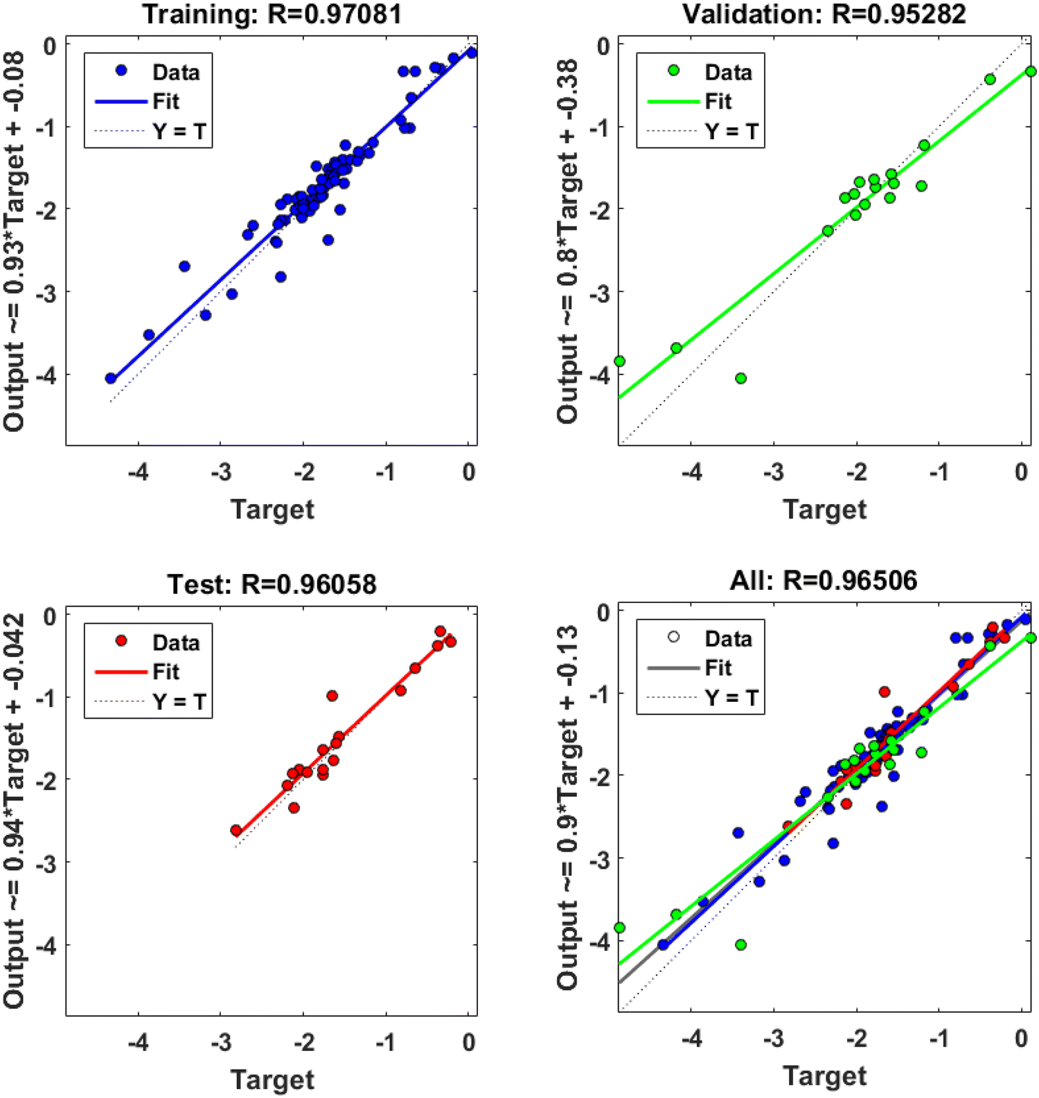
Figure  ² shows the comparison of experimental and predicted values for Logit (100- % CE) model for steam-assisted flares. The model in Fig.  ² uses NHV _CZ , S, U/V, U, CHR, CN, and D as inputs that can be used only when gas composition analysis can be done through the spectroscopy. Figure  ³ shows the comparison of experimental and predicted values for Logit (% Opacity) models for steam-assisted flares. Logit opacity model uses NHV _CZ and U/V in the model used in Fig.  ³ . Both Logit models for opacity and CE have a correlation coefficient of greater than 0.97. Figure  ⁴ shows model for assisted steam data as Log(S) as output against experimental data. 70% data is used in training and 15% each is used in validation and testing in all the models. 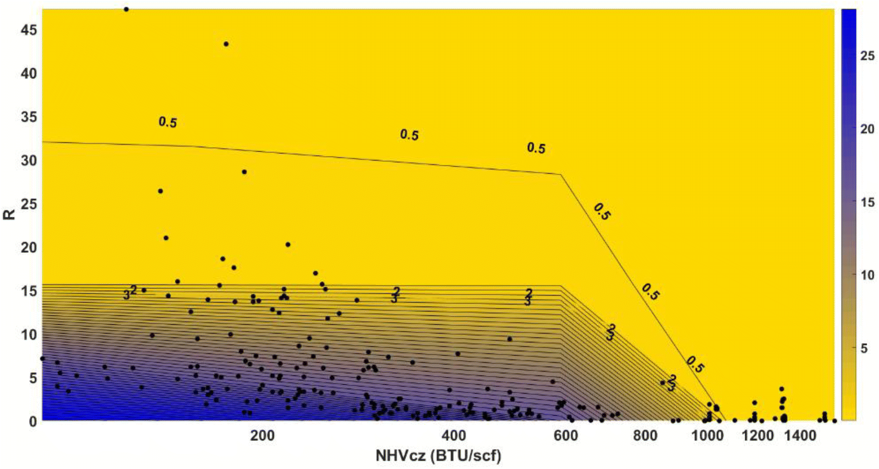Figure  ⁵ shows the contours of CE on R vs NHV _CZ at a fixed D (2 ft), S (110 lb/MMBTU) and U (8 ft/s) values. From Fig.  ⁵ it was observed that there is almost no flame at very low R and low NHV _CZ . With an increase in R at lower NHV _CZ (100-1000 BTU/scf), the CE was found to be high (90%). For all R beyond 15, the model predicted a good CE at the given S and U values. Figure  ⁶ shows the contour plot for Opacity over NHV _CZ vs R. The dark region represents highly smoking flare while the light regions represent very low to no sooting flare. The contour lines of 2% (SLF) and 3% (ISP) Opacity can be seen in Fig.  ⁶ . This plot demonstrates that at NHV _CZ below 1050 BTU/scf and R below 15, the opacity is very high. At R greater than 15, smoke is reduced. This is the same R value beyond which CE increases simultaneously as seen in Fig.  ⁵ .

Fig. 2

Fig. 3

Fig. 4

Fig. 5

Fig. 6

Air-assisted flare models

Figures  ⁷ and ⁸ show the comparison of experimental and predicted values for Logit (100- %CE) and Logit (%Opacity) models, respectively, for air-assisted flares. Figure  ⁹ shows the inverse model for air assist (Log A) as an output between the predicted and experimental data.

Fig. 7

Fig. 8

Fig. 9

The final model summary for air-assisted flare tests data, containing the response and input variables, number of neurons used, the calculated variance (VE %), MAE % and the correlation coefficient, r is shown in Table  ⁴ .

Table 4

Response	Input	# Neurons	R	MAE (%)	VE (%)	GC measurement required?
Logit (100- %CE)	U, V, A, NHVdil, D	5	0.95	1.17	88.23	No
Logit (100- %CE)	R, A, NHVdil, D, CHR	2	0.95	1.08	89.98	Yes
Logit (%Opacity)	U, V, A, NHVvg, D	6	0.96	1.75	91.71	No
Logit (%Opacity)	U, V, A, NHVvg, D, CHR	4	0.98	0.79	96.46	Yes
Log A	NHVvg, NHVdil, Logit(%Opacity)	3	0.96	–	93.34	No

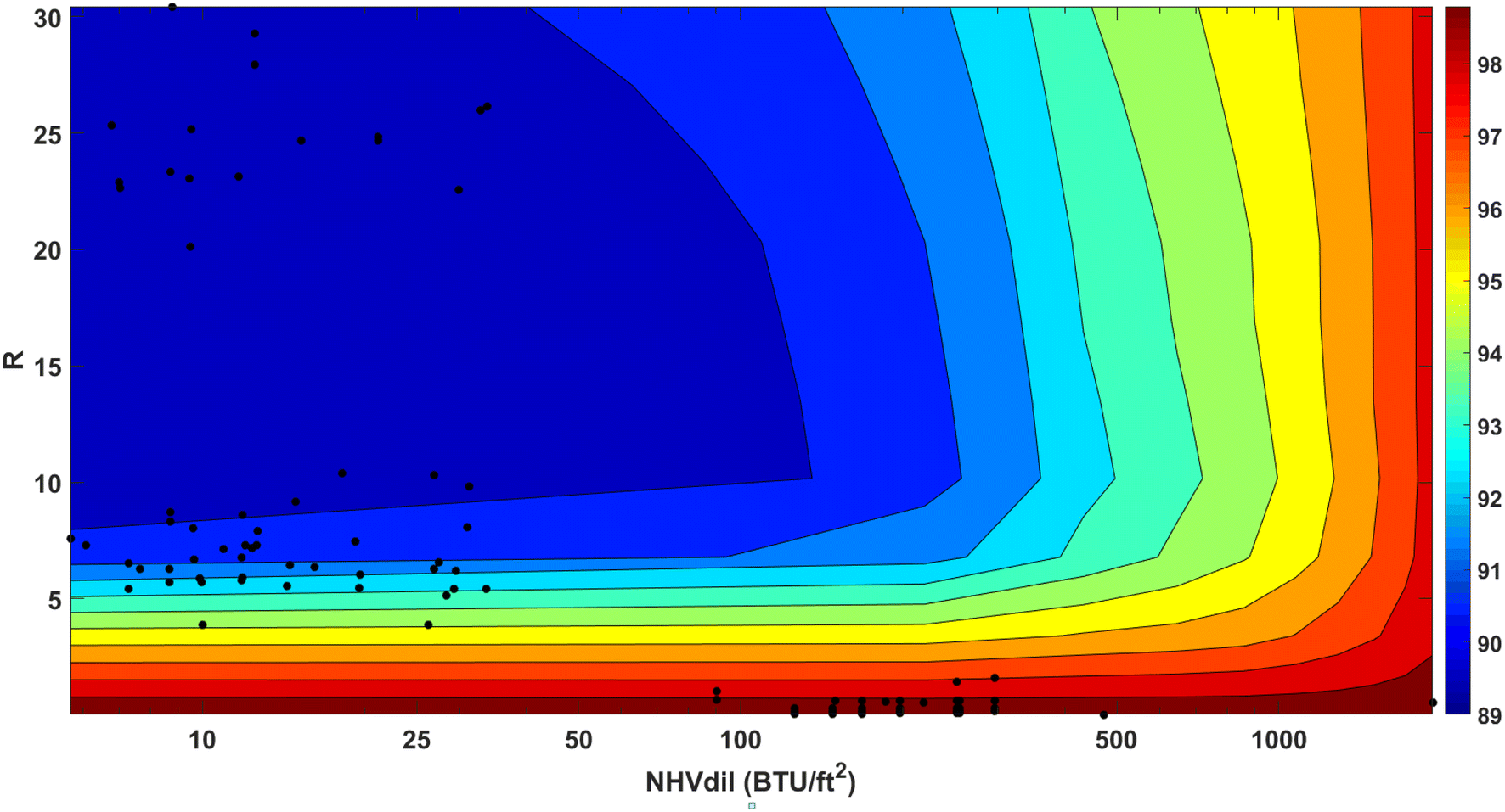
Figure  ¹⁰ shows the contours of CE on R vs NHV _dil at a fixed D (1.5ft), A (8000 lb/MMBTU), and CHR (0.4) values. The same plot can be drawn at a different set of values but it’s important to choose typical values, like middle of the range or near ISP values to show the trends of the models. From Fig.  ¹⁰ , it is seen that CE is high at low R but decreases sharply (99% to 89%) with increase in R, at lower NHV _dil (< 100 BTU/ft ² ). CE is found to be high (97%) for NHV _dil greater than 1200 BTU/ft ² for all R. Figure  ¹¹ shows the contours of CE over A vs NHV _dil at a fixed D (1.5ft), R (15) and CHR (0.4) values. From the trend of the contours it is observed that over-aeration leads to low CE especially at lower NHV _dil and at high NHV _dil , CE can still be high until 16,000 lb/MMBTU of air assist, beyond which the efficiency drops. Contour plot for Opacity over NHV _vg vs A is shown in Fig.  ¹² . The dark region represents a highly sooting flare while the lighter regions represent a very low sooting to smokeless flare. Of the 5 input variables of opacity model, D (1.5ft), V (1ft/s), and U (10ft/s) have been fixed. The contour lines of 2% (SLF) and 3% (ISP) Opacity can be seen in Fig.  ¹² . This plot confirms that over-aeration not only decreases CE but also makes the flare smokier, particularly at low NHV _dil /NHV _vg .

Fig. 10

Fig. 11

Fig. 12

All the performance criteria (r, VE, MAE) were calculated for the original variables (% CE or % Opacity) from the logit functions of models by converted back. These results indicated that there was a good agreement between the experimental and predicted values. Artificial neural network models developed in this study can be used further to determine the amount of air/steam assistance to achieve the desired CE. NN models presented in this study confirm the considerable value of the NN based approach in predicting the flare performance.

Application of the NN models for flare setpoint determination

Current control practices only address opacity to satisfy the EPA requirements. Operators tend to over-steam or over-aerate to suppress smoke at the expense of combustion efficiency (CE). Stand-by mode operations with low vent gas flow rates and low heating values often lead to (Destruction Removal Efficiency) DRE/CE below their expected values of 98%/96.5%. Refineries need to monitor and maintain minimum combustion zone net heating value (NHV _CZ ) as per EPA’s flare MACT rule [ ²⁰ , ⁵³ ]. Incipient smoke point (ISP) is widely recognized as the condition for most efficient burning. Determining the setpoints for flare operations at ISP and Smokeless flaring (SLF) operations is a major criterion to make flares compliant with the EPA regulations. Determining the setpoint (amount of steam/air/make-up fuel required) at the ISP and for smokeless flaring (SLF) has been performed as a part of this study. Desirable operating inputs can be set for the ISP (NHV _dil  ≥ 22 BTU/ft ² & Opacity ≤ Opacity _ISP ) and for smokeless flaring with NHV _dil  ≥ 22 BTU/ft ² and Opacity ≤ Opacity _SLF . The definitions of NHV _CZ and NHV _dil have been shown in Eqs.  ³ and ⁴ , respectively [ ¹⁶ ].

The criteria for air-assisted flares at the ISP is determined as NHV _dil  ≥ 22 BTU/ft ² and Opacity = 3% and for smokeless flaring is NHV _dil  ≥ 22 BTU/ft ² and opacity = 2% [ ⁵⁵ , ⁵⁶ ]. The same criteria for steam-assisted flares at the ISP is determined to be NHV _CZ  ≥ 270 BTU/scf and Opacity = 3% while for smokeless flaring the criteria is NHV _CZ  ≥ 270 BTU/scf and Opacity = 2%. The developed NN models have been used at the ISP and SLF to determine the operation set points in compliance with the current EPA regulations. The specific set point of a manipulated variable (steam-/air-assisted or make-up fuel or NHV _CZ ) was solved by specifying opacity and NHV _CZ  ≥ 270 BTU/scf or NHV _dil  ≥ 22 BTU/ft ² for steam- and air-assisted flare data, respectively [ ⁵⁵ , ⁵⁷ ]. For cases that do not satisfy the minimum heating value requirement, make-up fuel needed to be added to increase it to the minimum required value (NHV _CZ  = 270 BTU/scf or NHV _dil  = 22 BTU/ft ² . Natural gas (NHV _f  = 914 BTU/scf) is generally used as the make-up fuel for these gases.

Consider a steam flare:

Given NHV _vg is a measured disturbance variable, NHV _CZ  = 270 BTU/scf and opacity = 3% are specified at the ISP and the equations were solved in excel using the NN model equations to obtain the desired S, F, and NHV _CZ . The same methodology has been implemented to determine the make-up fuel and assisted steam/air for smokeless flaring, which has a lower opacity specification, 2%.

The model parameters for the ISP and SLF have been exported to excel and then solved using the methodology to find the assistance air required to achieve the specific criteria of NHV _dil  ≥ 22 BTU/ft ² and opacity = 3% at the ISP and NHV _dil  ≥ 22 BTU/ft ² and opacity = 2% for SLF. The opacity settings are based on the average % Opacity of the ISP characterization [ ²⁷ , ²⁸ ] and are used here for illustration purposes. Since states (or countries) have various definitions of % Opacity for smoky flares (visible emissions), users can adapt the numbers (e.g., 5%, 10%, etc. for % Opacity at the ISP) to comply with the regulatory requirements. Logit(100- %CE) model is then used to find the final CE at the ISP.

The predicted air assist, CE, and NHV _dil at the ISP has been compared against those for smokeless flaring (SLF) data in Figs.  ¹³ , ¹⁴ and ¹⁵ , respectively. Both NHV _dil and NHV _CZ have make-up fuel in the numerator and A or S in the denominator and hence will lead to multiple solutions satisfying the inequality constraints (NHV _dil  ≥ 22 BTU/scf or NHV _CZ  ≥ 270 BTU/scf). However, from the economic standpoint, i.e., to minimize the use of make-up fuel and steam (or air), Q _f  = 0 is always practiced.

Fig. 13

Fig. 14

Fig. 15

The predicted air assistance has been significantly lowered while increasing the NHV _dil and CE simultaneously for all the test cases. CE is found to be higher than the experimental data for all the test cases. None of the air-assisted flare tests required any external make-up fuel to determine the setpoints for ISP or for SLF. For cases where make-up fuel would be required, it is important to add the make-up fuel into the calculation of NHV _{vg, req} since NHV _{vg, req} will become the new NHV _vg for further calculation of required steam and CE till convergence. The make-up fuel used in the SP determination is natural gas to increase the net heating value of the vent gases.

The ISP characterization results by Chen et al. for steam-assisted flares show that about 16–211 lb/MMBTU of steam and 342–1374 BTU/scf of NHV _{vg, req} at the ISP whereas the NN model recommends 0–94 lb/MMBTU of steam and NHV _{vg, req} is the same as the experimental NHV _vg (348–2350 BTU/scf). Similarly, the ISP characterization results for air-assisted flares show that about 4431–8609 lb/MMBTU of air and 297–1157 BTU/scf of NHV _{vg, req} at the ISP whereas the NN model recommends 0 to 5900 lb/MMBTU of assisted air and NHV _{vg, req} is the same as the experimental NHV _vg (339–2117 BTU/scf). Table  ⁵ summarizes the comparison of assistance steam/air predicted by NN model against the values determined by ISP characterization by Chen et al. [ ²⁸ ]. The formula to calculate NHV _{vg, req} is given as follows:

For the steam-assisted flare tests, the setpoints at the ISP and at SLF were determined using the same methodology. Figs.  ¹⁶ , ¹⁷ , and ¹⁸ show predicted steam assist, % CE and NHV _CZ , respectively, at the ISP vs SLF. All the steam cases required no make-up fuel to meet the criteria at ISP/SLF.

Fig. 16

Fig. 17

Fig. 18

While over-steaming/aeration can suppress smoke, it is usually at the expense of combustion efficiency and this has been demonstrated both by the setpoint results and the contour plots of CE and Opacity. The discrepancy between the predicted ISP steam/air/make-up fuel and experimental data can be justified: First, the observed ISP are not very rigorous due to human observation errors as seen by the wide variations in characterized ISP opacity, combustion efficiency, heating value, etc.; Secondly, the ISP or SLF can be achieved in multiple states by simultaneously increasing NHV _{vg, req} (NHV _vg and make-up fuel) and the diluent (steam and air assist) for better air mixing. Therefore, ISP or SLF can be achieved by simultaneously introducing make-up fuel and steam or by reducing steam (or air) alone. Even though adding no make-up fuel is the priority in the solution algorithms, it will be interesting to compare the solution of the minimization of fuel and steam/air use and maximization of combustion efficiency (CE) to the present work.

Conclusion

Artificial neural network (ANN) models that showed good correlation coefficients between experimental data (controlled flare tests from 1983 to 2014) and model predictions were developed for both steam- and air-assisted flares. The models included performance models for opacity, combustion efficiency (CE), and operation models for assistance steam and air. Input variables include NHV _vg , S, A, NHV _CZ , NHV _dil , D, V, U, CN, and CHR, where carbon to hydrogen atomic ratio (CHR) and carbon number (CN) reflect vent gas species effect and NHV _CZ and NHV _dil are parameters that combine the effect of steam/air assists and vent gas heating value NHV _vg to facilitate easy flare control. NN models for steam- and air-assisted flare tests have shown a good agreement with experimental data and this has been demonstrated by the average correlation coefficient being 0.95 and 0.97 for air-assisted and steam-assisted flare data, respectively. The mean absolute errors of 1.1% and 1.4% for air-assisted and steam-assisted flare data, respectively also confirm the performance and robustness of the NN models. As shown in Table  ⁵ it can be stated that NN predictions at the ISP are in good agreement and well within the boundaries set by the ISP characterization paper. The 2-D contour plots have been presented to show the trends of the important parameters emphasizing the interaction between % CE, % Opacity, and assistance air/steam.

Specific set points of the controllable variables like steam/air assist and make-up fuel were determined using ANN that satisfies stipulated NHV _CZ  ≥ 270 BTU/scf (for steam-assisted flares) or NHV _dil  ≥ 22 BTU/scf (for air-assisted flares) and opacity = 3% for the ISP and opacity = 2% (operating slightly below ISP) for SLF. Operating slightly below the ISP opacity should be most economical. The NN models built in this study demonstrated that by reducing the amount of air/steam used smokeless flaring can be achieved for vent gases with high net heating values while still complying with CE ≥ 96.5%. The models built are reliable to guide flare operations in compliance with regulations.