The Franconian Basin thermal anomaly: testing its origin by conceptual 2-D models of deep-seated heat sources covered by low thermal conductivity sediments
GeoZentrum Nordbayern, Friedrich-Alexander-University Erlangen-Nürnberg (FAU), Erlangen, 91054, DE
Gesteinslabor Dr. Eberhard Jahns, Heiligenstadt, 37308, DE
Abstract
This study presents conceptual 2-D models for coupled fluid flow and heat transport simulations of the Franconian Basin in SE Germany to verify the plausibility of different hypothesis on the origin of a local temperature anomaly. The simulated geothermal systems consist of a deep-seated heat source within an impermeable basement (heat-producing granite or enhanced background heat flow), covered by low thermal conductivity sediments. Solely conductive or additional convective heat transport including the presence of a permeable fault was applied. We found that heat transfer in the model setups is strongly controlled by (1) the volume of the heat-producing granite, (2) the amount of the background heat flow, (3) the permeability of the basement rocks, (4) the thermal conductivity contrasts between the sedimentary cover and the basement, and (5) the type of heat transport. If there is no reliable information on these model parameters, a high degree of uncertainty with regard to quantitative statements on the heat transfer in the specific geothermal system can be expected. An equilibrium temperature log from the study area could only be reproduced by (1) an enhanced background heat flow of 0.115 W m
−2
, in combination with a permeable fault zone of permeability 1.0 × 10
−13
m
2
or (2) a heat-producing granite of large cross-sectional area (300 km
2
) in combination with an average background heat flow of 0.070 W m
−2
. Moreover, high temperatures were only achieved in the presence of a low conductive, insulating cover above the heat source.
Introduction
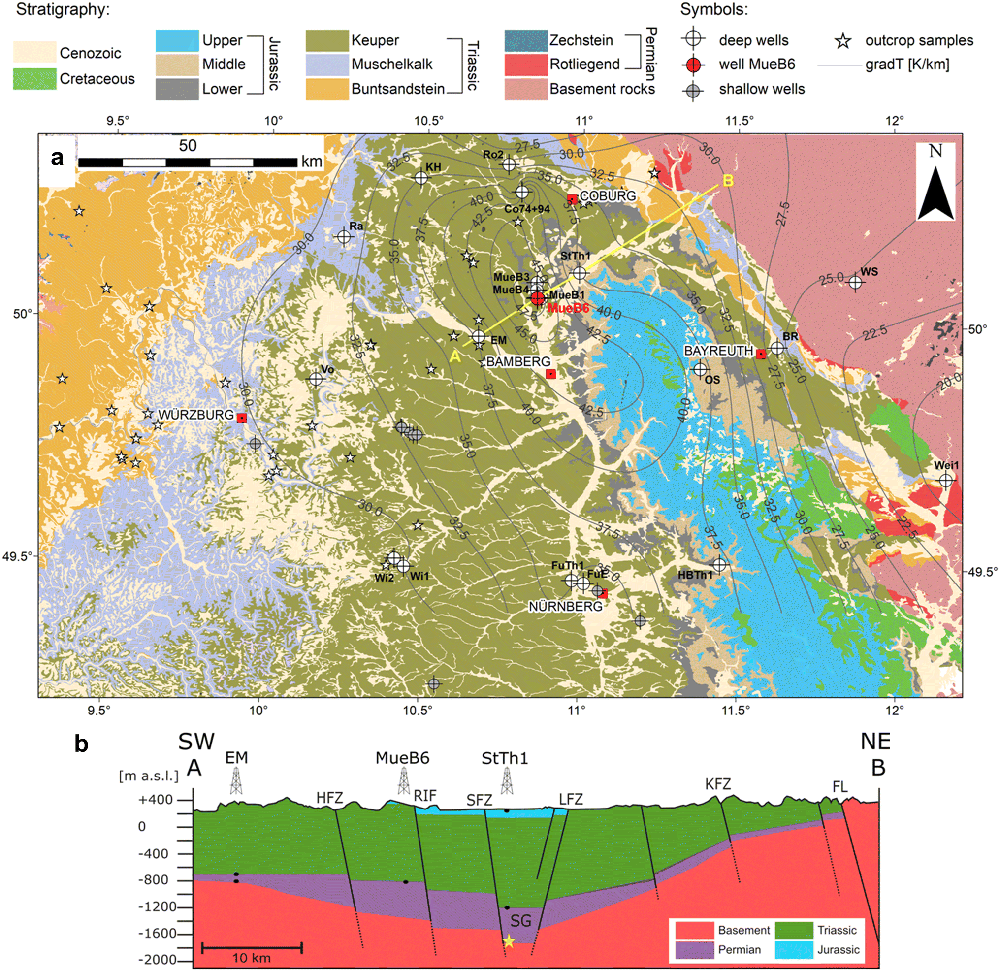
The existence of a positive temperature anomaly in the Franconian Basin (SE Germany) (Fig.
1
) has been verified since the 1980s. It covers an area of ~ 100 × 65 km
2
(Fig.
2
a), with a maximum geothermal gradient (grad
T
) of 48.9 K km
−1
over a depth interval of 1200 m [
1
,
2
–
3
]. However, the geological cause(s) of the anomaly are not yet clear. Also, it is not proven whether the elevated temperatures already occur in the basement or whether they are limited to the sedimentary cover. In the first case, the Franconian Basin would harbour a hitherto unknown petrothermal potential. Petrothermal reservoirs are classified as very reliable sources of energy with high heat content and bear the highest future potential [
4
,
5
–
6
] although the technology is much less developed compared to hydrothermal systems and also more expensive to exploit [c.f.,
5
,
6
].
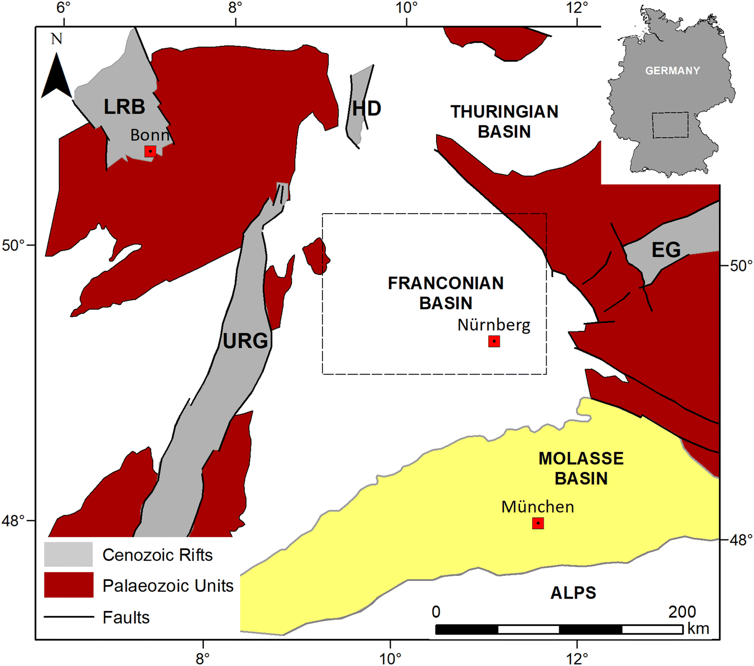
Fig. 1
Large-scale structural framework in the periphery of the Franconian Basin, including Palaeozoic units and parts of the European Cenozoic Rift System (ECRIS). The position of the study area is indicated by the dashed frame
Fig. 2
a
Geological map of the Franconian Basin, showing locations of deep wells and grad
T
contour lines of the Mürsbach temperature anomaly (supplementary Appendix A for well data and abbreviations). Geology compiled from [
77
,
78
,
79
,
80
,
81
–
82
];
b
schematic geological NE-SW cross section illustrating the basement topography and the general structural and stratigraphic framework of the case study area (10 times vertical exaggeration). The position of the geological cross section is illustrated by a yellow line in
a
. Black dots: deep-well verified formation tops; yellow star: basement top interpreted from DEKORP-3B section [
44
]
Various hypothetical underground scenarios are currently under discussion as potential reason(s) for the elevated temperatures in the Franconian Basin: (1) heat-producing granites within the basement, (2) the presence of deep, hydraulically active fault zones [
7
], and/or (3) elevated heat flow due to the proximity to European Cenozoic Rift system (Fig.
1
) [c.f.,
8
–
10
] and the associated cenozoic magmatism [
1
,
11
]. However, none of these hypotheses can be proven directly by reliable field data. While the structural framework of the sedimentary cover in the centre of the anomaly is relatively well known from deep wells, there is little sincere information about the basement depth, lithology, structure and hydraulic activity.
At this stage of knowledge, the use of thermo-hydraulic simulations is a useful tool to test the plausibility of different hypotheses for the local subsurface configuration, as this method provides the possibility of merging data from different scales. For example, numerical modelling provides an opportunity to quantify the thermal impact of specific heat sources such as elevated heat flow from the Earth’s interior or radioactive granites. The vast number of existing numerical models on granites mainly deals with the thermodynamic processes associated with granite formation and emplacement [
12
,
13
–
14
], the simulation of fluid flow in fractured granite reservoirs [
15
,
16
–
17
] or the cooling process of plutons and its effects on the surrounding host rocks [
18
,
19
–
20
]. Although there are a few studies dealing with different heat production rates of deep-seated granites below a low thermally conductive cover [
21
,
22
], there are no systematic studies quantifying the impact of their volume and absolute depth on the temperature distribution in the overburden. Thermal models quantifying the impact of different values for the average heat flow from below (mainly generated by radioactive decay in the mantle and the crust) are also missing.
In this study, we perform coupled fluid flow and heat transfer simulations in conceptual 2-D models that depict various potential subsurface configurations for the subarea of the Franconian Basin in SE Germany, which is identified to host the central part of the thermal anomaly outlined above. The modelled geothermal system consists of a deep-seated heat source within an impermeable basement covered by low thermal conductivity sediments. The system can be classified as basement/crystalline rock type geothermal play type [
23
]. The focus of the study is on the quantification of the impact of different model variables on the temperature distribution in the tested geothermal system, namely:
different volumes and depth levels of a heat-producing pluton,
different values of the average heat flow from below,
the effect of different heat transfer modes (conductive vs. convective),
the variability of the permeability value of the basement layers and,
the impact of the implementation of a variably permeable fault zone.
The comparison of the modelled temperature profiles with the existing present-day thermal field in the centre of the thermal anomaly then allows the assessment of the plausibility of specific scenarios discussed as potential causes for the local temperature high.
Since the temperature distribution in the crust, in addition to the distribution of radioactive elements, is mainly controlled by the thermal conductivity of rocks [
24
,
25
], statistically validated thermo-hydraulic data of the sedimentary key strata and the basement rocks were measured in the course of this study and used for model calibration (Table
1
).
Table 1
Stratigraphic chart and thermo-hydraulic input parameters of the models presented in this study
Depth (m)
Stratigraphy
Lithology
n
λ (W m−1 K−1)
a (mm2 s−1)
ρbulk (kg m−3)
Φ
Cp (J kg−1 K−1)
k (m2) (n)
Reference rock properties
Model layer
Triassic
Keuper
81.5a
Hassberge-F [84]
kmBL i.w.S [84]
Sst
67
3.2
1.5
2202
0.19
969
1.3 × 10⁻¹⁴ (8)
This study
1
Clst/Slst
–
2.1
1.0
2500
0.08b
840
1.0 × 10⁻¹⁶
[73], [88]
2
130.8a
Steigerwald-F [84].
kmL [84]
Clst
–
2.1
1.0
2500
0.08b
840
1.0 × 10⁻¹⁶
[73], [88]
3
174.3a
Stuttgart-F [84].
kmS [84]
Sst
61
2.6
1.2
2237
0.14
969
1.2 × 10⁻¹⁴ (40)
This study
4
286.3a
Benk-F [84].
kmE + kmM [84]
Clst
–
2.2
1.0
2500
0.08b
840
1.0 × 10⁻¹⁶
[73], [88]
5
338.3a
Grafenwöhr-F [84].
ku [84]
Clst/Dol
16
2.3
13
2418
0.13
732
1.0 × 10⁻¹⁶ (6)
This study
6
Muschelkalk
412.4a
Upper [83]
mo [85]
Ls
62
2.7
1.4
2646
0.02
729
2.4 × 10⁻¹⁶ (12)
This study
7
mrlst
–
1.8
0.9
2500
0.08b
800
1.0 × 10⁻¹⁶
[87], [88]
8
474.1a
Middle [83]
mm [85]
Ls
25
2.7
2.0
2866
0.02
471
2.0 × 10⁻¹⁶(5)
This study
9
549.0a
Lower [83]
mu [85]
Ls
12
2.6
1.5
2699
0.02
642
1.1 × 10⁻¹⁶(4)
This study
10
mrlst
–
1.8
0.9
2500
0.08b
800
1.0 × 10⁻¹⁶
[87], [88]
11
Buntsandstein
Upper (Röt-Fm. s7) [83]
so4T/so3T [85]
Clst
–
2.1
1.0
2500
0.08b
840
1.0 × 10⁻¹⁶
[73], [88]
12
so4Q [85]
Sst
11
4.7
2.1
2428
0.09
922
2.4 × 10⁻¹⁴ (4)
This study
13
632.0a
so2P [85]
Sst
122
3.4
1.4
2479
0.08
980
5.2 × 10⁻¹⁵ (7)
This study
14
747.9a
Middle (s3–s6) [83]
sm [85]
Sst
71
3.8
1.5
2402
0.10
1055
3.3 × 10⁻¹⁵ (11)
This study
15
Clst
–
2.1
1.0
2500
0.08b
840
1.0 × 10⁻¹⁶
[73], [88]
16
1058.6a
Lower (s1–s2) [83]
su [85]
Sst
105
3.7
1.6
2350
0.11
984
3.9 × 10⁻¹⁵ (15)
This study
17
Clst
–
2.1
1.0
2500
0.08b
840
1.0 × 10⁻¹⁶
[73], [88]
18
Permian
Zechstein
1079.7a
Fulda-F. (z7) [83]
Clst/Sst
23
3.0
1.3
2500
0.08b
985
1.0 × 10⁻¹⁶
This study
19
1082.9a
z6–z4 [83]
Clst/Gyp
2
3.2
1.1
2500
0.08b
1164
1.0 × 10⁻¹⁶
This study
20
1086.0a
Leine-F. (z3)
zLAN [86]
Anhy
4
5.1
2.2
2923
0.01
793
7.4 × 10⁻¹⁷ (3)
This study
21
1092.3a
zLCA [86]
Dol
7
4.0
1.6
2833
0
882
1.2 × 10⁻¹⁵ (2)
This study
22
1096.8a
Staßfurt-F. (z2)
zS [86]
Clst/Dol
3
2.5
1.2
2500
0.08b
833
1.0 × 10⁻¹⁶
This study
23
1100.2a
Werra-F. (z1) [83]
zWANo [86]
Anhy
10
4.8
1.9
2937
0.01
860
5.6 × 10⁻¹⁷ (4)
This study
24
1111.8a
zWTo [86]
Clst
–
2.1
1.0
2500
0.08b
840
1.0 × 10⁻¹⁶
[73], [88]
25
1114.9a
zWANu [86]
Anhy
9
4.9
2.2
2904
0.01
767
5.6 × 10⁻¹⁷ (4)
This study
26
1164.2a
zWCAR [86]
Dol
54
4.3
1.5
2800
0.04
1024
1.8 × 10⁻¹⁶ (11)
This study
27
1201.3a
zWCA [86]
mrlst
14
2.3
1.2
2933
0.01
653
3.2 × 10⁻¹⁶ (2)
This study
28
1400.0
Rotliegend, unclassified
Sst
18
3.4
1.5
2589
0.03
932
3.6 × 10⁻¹⁶ (6)
This study
29
Cgl
6
3.0
1.2
2660
0.03
940
1.5 × 10⁻¹⁵ (6)
This study
30
Mean (sedimentary cover)
–
2.8
2470
7400.0
Basement
Phyllites (d = 6000 m) [46]
23
3.7
1.9
2700
0
721
1.0 × 10⁻¹⁸
This study
31
9900.0
Paragneiss 1 (d = 2500 m) [46]
–
3.5
1.7
2720
0
757
1.0 × 10⁻¹⁸
[20], [89]
32
17,000.0
Paragneiss 2 (d = 7100 m) [46]
–
3.4
1.7
2750
0
727
1.0 × 10⁻¹⁸
[20], [89]
33
20,000.0
Middle crust (d = 3000 m) [46]
–
2.6
1.5
2960
0
586
1.0 × 10⁻¹⁸
[20], [90]
34
–
Granite
–
3.4
1.7
2600
0
769
1.0 × 10⁻¹⁸
[89]
–
The following “
Case study area
” presents the regional geological framework of the case study area, including available temperature data as well as the measured thermo-hydraulic input data. “
Model setup
” then presents in detail the structure of the basic 2-D model, the basic model parameterization and the modelled scenarios and variables, which are subsequently discussed in “
Results and discussion
”.
Case study area
Geological framework
The temperature anomaly of interest is situated within the Franconian Basin [
26
] in SE Germany (Fig.
1
). The basin is underlain by Saxothuringian Variscan basement [
27
] and comprises Permian, Mesozoic and Cenozoic sedimentary rocks, with sandstones, siltstones, claystones, carbonates and few evaporites forming the prevailing rock types. The sedimentary cover reaches a thickness of > 1600 m in the Staffelstein Graben [
28
] NW of well Mürsbach B6 (MueB6) (Fig.
2
b). Upper Triassic sediments of the Keuper unit dominate the surface outcrops in the study area Fig.
2
a).
The basement geology of the Franconian Basin was formed during the amalgamation of Western Europe during the Variscan Orogeny accompanied by the intrusion of numerous voluminous granites [
27
,
29
,
30
]. During the Cenozoic, the study area was affected by the development of the European Cenozoic Rift System, which involves the emplacement of Eocene to Pleistocene alkaline and minor tholeiitic intraplate basalt dikes [
31
,
32
] and adjacent to the study area, the formation of NW and NE striking rift basins.
NW–SE and NE–SW striking faults dominate the regional structural framework, some of which reflecting deep-seated basement faults that experienced multiple reactivation [
33
,
34
]. Permeable and deep-reaching fault zones in the study area are indicated by locally enhanced radon emanations [
35
]. Such hydraulic basement connections can be assumed especially for the areas of intersection of NW–SE to NNW–SSE striking faults [
36
], which are orientated (sub)parallel to the recent stress field [
37
].
Temperature data
All available well data, including temperature readings of deep wells in the case study area are summarised in supplementary Appendix A.1 and A.2. The highest temperature of 66.8 °C at 1204.2 m depth in the centre of the temperature anomaly was recorded by the
T
-Log1_MueB6 (name given for this study) in the deep well MueB6 [
3
] (Fig.
2
a). The temperature log is interpreted to provide undisturbed formation temperatures, as the shut-in time of 18 months (supplementary Appendix A.1) is considered as a sufficient time period to reach complete thermal equilibration after drilling and mud circulation were completed [
38
,
39
].
Thermo-hydraulic input data
The presented models were calibrated using geologically and statistically valid thermo-hydraulic data of the Franconian Basin in SE Germany. 509 core samples were collected from the deep wells (> 400 m) Obernsees 1 (OS), Mürsbach B1, Mürsbach B3, Mürsbach B4 (Fig.
2
a), and also from several shallow wells (Fig.
2
a, 163 cores), reaching down to 20–40 m depth. To include stratigraphic units that could not be sampled from cores, additional outcrop samples (
n
= 53) were collected (Fig.
2
a). Because of restricted sample availability of particular formations (e.g., clay- and marlstones of the Upper and Middle Triassic), published thermal–hydraulic data had to be integrated (Table
1
).
Measurements were performed for the main rock types of almost all stratigraphic units of the Permo-Triassic sedimentary cover as well as for selected Variscan basement rocks (Table
1
). The input parameters of the models presented are thermal conductivity (
λ
), thermal diffusivity (
a
), bulk density (
ρbulk
) porosity (
Φ
) and specific heat capacity (
Cp
). For convective models, the permeability (
k
) was added as a variable.
Cp
was calculated from the measured
λ
,
ρbulk
, and
a
.
Thermo-hydraulic data of basement rocks could only be measured on core material of well OS (Fig.
2
a). No additional basement core material was available from any other deep wells within the study area due to its restricted exploration status.
Thermal conductivity and thermal diffusivity
Thermal conductivity (
λ
) and thermal diffusivity (
a
) measurements were performed on water-saturated (deionised water) samples at ambient conditions (22 ± 2 °C, atmospheric pressure). We applied the optical scanning method (thermal conductivity scanner TCS; Lippmann and Rauen GbR) introduced by Popov et al. [
40
], giving an accuracy of ± 3%. The measured
λ
and
a
values of the sedimentary cover show broad ranges of 1.8–4.3 W m
−1
K
−1
and 1.0–2.2 mm
2
s
−1
, respectively.
For technical reasons, we uniformly used petrophysical values, measured parallel to the orientation of the sedimentary bedding planes. Due to negligible tectonic tilting and the subvertical orientation of the wells, sedimentary bedding in all core samples is oriented ± perpendicular to the c-axis of the cores. Measurements of
λ
and
a
, performed on the flat surfaces of slabbed core samples, then represent values from a subparallel orientation of the sedimentary bedding planes in relation to the measurement signal.
Porosity, bulk density and permeability
For the determination of
Φ
and
ρbulk
, the Archimedes’ principles was applied on plug samples (
n
= 661,
Ø
= 29 mm;
L
= 45 mm), which were drilled from core and outcrop samples. For another 384 core samples, whole core measurements have been performed. To avoid clay mineral swelling and the damage of the mineral lattice, isopropanol was used as saturation fluid.
Φ
and
ρbulk
values range between < 1 and 19%, with bulk rock densities of 2100 to 2866 kg m
−3
(Table
1
). Air-permeability, calculated by Darcy’s law, was also measured on plug samples (
Ø
= 29 mm;
L
= 45 mm) using a Hassler cell and following the measurement procedure described by Filomena et al. [
41
].
Model setup
Software
For numerical modelling, the heat transfer module and subsurface flow module of the FEM software package COMSOL Multiphysics
®
5.3a (known as FEMLAB prior to 2005; [
42
]; Comsol Multiphysics:
https://www.comsol.de
, accessed 08/02/2019) were used. The software allows modelling of conductive heat transfer in porous media as well as convective Darcy flow of fluids within permeable rocks and fractures.
As the fluid properties exert a major control on the heat transport within a system [
43
], the thermo-physical parameters of the fluid (
λ
, density, viscosity) had to be adjusted to ambient temperature conditions. The governing equations used in this study are provided in supplementary Appendix B. Specific software settings applied during the numerical simulations are provided in Table
2
.
Table 2
Specific software settings of the numerical simulations with COMSOL Multiphysics
®
Meshing
Free triangular meshing
Number of elements
692,585a
COMSOL element size
Finer
Element sizeb
2.4 − 1.7 × 10³ m
Heat-production of granite
Constant (start heating at 0 Ma)
BHT (lower boundary)
Constant
Solver
Time-dependent, MUMPS
Simulation time
300 Ma
Solver maximum step
0.1 a
Tolerance factor
0.1c
Time-stepping-method
BDF (backward differentiation formula)
Tested subsurface configurations
We have tested four conceptual 2-D subsurface configurations, which differ in the type of heat source, the presence or absence of a permeable fault and the type of heat transport (purely conductive or combined with an additional convective transport component). The two different heat sources are:
Various values for the average heat flow from below (generated by radioactive decay in the mantle and the crust as well as from cooling of the residual heat from the time of Earth’s origin). This is referred as background heat flow (BHT) in this study.
Variable volumes of a heat-producing granite, representing an additional radioactive heat source (besides the BHT) in the crust.
For applying a pure conductive thermal regime, the two tested subsurface configurations are:
The basic model (B-model), in which various values for the background heat flow (BHF) of 0.070–0.125 W m
−2
are applied as the only heat source at the lower boundary of the model (Fig.
3
a, Table
4
). A BHF value of 0.070 W m
−2
generates a temperature–depth profile expectable from a normal continental geothermal gradient of 30 K km
−1
in the B-model setup.
Fig. 3
Conceptual model setup
a
of the four tested underground configurations
b
of the BGF-model in more detail. The analysed (exported) model temperature profile
P
is indicated by the dotted line
The basic model with granite (BG-model), in which a heat-producing granite body provides an additional heat source to the BHF (Fig.
3
a, Table
4
). In this model setup, the BHF is not varied and uniformly set to 0.070 W m
−2
.
The setup of the B-model was calibrated on the stratigraphic data of the deep well MueB6, for which the equilibrated
T
-Log1_MueB6 is available and where the highest underground temperatures in the study area were measured (Fig.
2
a). The simulations presented do not provide a basin-scale study, but only depict the central region of the temperature anomaly in the Franconian Basin. The stratigraphy of the sedimentary cover in well MueB6 and measured thermo-hydraulic characteristics of the sedimentary rocks (Table
2
) are valid for this part of the basin.
As the model area in numerical modelling is of finite extension, it is important that it is large enough not to influence the resulting temperature distribution. In our model setup, the total model depth
zmodel
defines the vertical distance between the heat source at the lower boundary (BHF) and the surface of the model. In addition,
zmodel
controls the thickness of host rocks around the pluton in the model setup comprising a heat-producing granite (Fig.
3
b). Therefore, in a first step, sensitivity analyses of both parameters were performed, in order to determine the minimum model depth and width required not to influence the resulting temperature distribution (“
Model extensions
”).
The sedimentary cover in the B-model (Fig.
3
a) is further subdivided into 30 layers of different thicknesses and rock properties, mirroring the main rock types and individual stratigraphic subunit thicknesses of well MueB6 (Table
1
). The lateral thicknesses of the layers are kept constant, considering a simplified “layer cake” stratigraphy, particularly of the Triassic. In the software; each layer was assigned the specific thermo-hydraulic parameters according to Table
1
.
As drilling of the adjacent well Mürsbach B1 ceased at 1309.0 m within the Lower Permian (Rotliegend), the exact depth of the basement-cover boundary is not known at the location of well MueB6 and only estimated at c. 1350–1400 m from the nearby DEKORP-3B section [
44
]. Well OS, located at the
E
′ border area of the Franconian Basin, reached Variscan metasedimentary basement rocks at a depth of 1341.7 m [
45
]. As the deep wells at the location Mürsbach are situated more towards the centre of the sedimentary basin, basement rocks are assumed at a greater depth compared to the location of well OS. In all model configurations, we uniformly set the top of the basement rocks at 1393.0 m assigning the Lower Permian a total thickness of 175 m.
In the B-model, the basement is subdivided into four sublayers (Fig.
3
b; Table
1
). The subsurface structure of the upper (Variscan) crust is assumed to be composed of 6000 m metapelites (Phyllite) and of 2500 m gneiss (Paragneiss 1) at the base. The upper crust is then underlain by about 7000 m of higher metamorphic grade Cadomian gneisses (Paragneiss 2) [
46
]. The thermo-hydraulic input parameters for the upper Phyllite layer were calibrated on core measurements of the well OS. Due to the lack of appropriate data for the lower basement layers, the input parameters were taken from the literature (Table
1
).
In order to test the effect of additional convective heat transport in the two basic model setups, we incorporated a permeable fault zone and also allowed convective heat transport in the pore space of the sedimentary cover. The permeability of the basement rock layers was kept at a low level, ensuring only conductive heat transport in this part of the model. The resulting convective model setups are the following:
The basic model with a fault (BF-model) (Fig.
3
a).
The basic model with granite and a fault (BGF-model) (Fig.
3
a, b).
As it is known that the permeability and the opening width of a fault have a significant impact on the hydrothermal field [
47
], sensitivity analyses were performed for this two parameters. In addition, the influence of the maximum depth extent of the implemented fault zone was tested.
Initial and boundary conditions
A constant surface temperature of 9.0 °C was applied as upper boundary condition (Fig.
3
b), which represents the mean annual air temperature in the centre of the case study area (CDC-FTP-Server Deutscher Wetterdienst:
ftp://ftpcdc.dwd.de/pub/CDC/
, accessed 14/01/2018). As lower boundary, the BHF was set. So-called infinite element domains were chosen as lateral boundaries (Fig.
3
b). According to COMSOL Multiphysics
®
, they give the model infinite lateral extension and prevent that the model results are influenced by the lateral model boundaries. The boundary conditions on the outside of the infinite element (thermal insulation) are effectively applied at a very large distance from any region of interest.
The lower and upper model boundaries are set impermeable with respect to flow. Absolute pressure in the model domains is set as pressure gradient, calculated from the specific depth, the density value of the model layer (Table
1
) and gravitational acceleration.
We only applied a
T
-correction of thermal conductivity (
λ
) data according to Somerton (1992) [
48
] (Eq.
1
), as the temperature effect dominates the pressure influence on
λ
values [
48
,
49
–
50
]:
λ(T)=λ20-10-3(T-293)(λ20-1.38)[λ20(1.810-3T)-0.25λ20+1.28]λ20-0.64.
Heat production and geometry of the granite
The heat-production rate of granites can vary over a broad scale. Heat-producing granites can be classified as low-, moderate- and high-heat-producing granites [
51
]. In this study we assume a moderate heat production (
Agranite
) of 6 μW m
−3
based on the data of Scharfenberg et al. [
52
] for the Fichtelgebirge and Oberpfalz granites, considered as surface analogues for the deeply buried granites in the study area. There, gravimetric modelling indicates the presence of isolated granite bodies within the buried Saxothuringian basement of the Franconian Basin, located at 2–18 km depth [
53
].
Besides the
Agranite
value, also the geometry and the cross-sectional area of granite bodies exert a control on the subsurface temperatures. Different pluton aspect ratios (length/thickness) are proposed in the literature. Dome and a sheet geometries are the two endmembers discussed [
54
,
55
]. We run our models with these two geometries, resulting in variable granite cross-sectional areas:
Tabular, sheet-like plutons have a power law geometry according to Eq. (
2
) [
54
,
55
], where
T
is the thickness of the pluton and
L
is its lateral extension. We tested two granite geometries in our 2-D models:
G
1 (11.55 km
2
) and
G
2 (35.0 km
2
) (Table
3
).
T=0.29L0.6.
Table 3
Modelled geometries and heat-production rate of the pluton in the BG- and BGF-model (Fig.
3
)
Name
Lateral extension (m)
Thickness (m)
Cross-sectional area (km2)
Reference geometry
Agranite (mW m−3)
Granite 1 (G1)
10,000
1155
11.55
a
6
Granite 2 (G2)
20,000
1750
35.0
a
6
Granite 3 (G3)
21,000
7000
147.0
b
6
Granite 4 (G4)
30,000
10,000
300.0
b
6
For the dome-shaped pluton geometry, we chose an aspect ratio of 3:1 (length/thickness). The tested geometries
G
3 and
G
4 have significantly larger cross-sectional areas (147.0 and 300.0 km
2
) than the tabular geometries
G
1 and
G
2, resulting in higher heat-producing granite volumes in the models.
To test the impact of the absolute pluton depth, the granite top was set to 2000, 4000 and 6000 m depth, respectively. For all model setups, we applied a time-dependent study with forward modelling of 300 Ma, an average of known granite emplacement ages in the Saxothuringian basement [
56
,
57
–
58
]. Heat supply by the granite and the BHT starts at 0 Ma, generating a transient temperature field at the beginning of the simulation. However, at constant heat supply by the heat sources, steady-state conditions are reached after 36 Ma at the latest. Although the tectonic configuration of the modelled part of the basin was not constant over the modelled period, the applied simulation time ensures that steady-state is always reached for all tested underground configurations. Questions regarding the history of the basin and tectonic aspects could not be implemented in the software and would go beyond the scope of the conceptual models presented.
Fault geometries and permeability
The magnitude of fluid flow within a permeable fault is directly related to its hydraulic and geometric aperture [
59
,
60
–
61
], which in nature can be very complex. However, for numerical modelling a planar fracture model with two smooth and parallel planes is commonly applied for simplification [
15
], representing a reasonable first-order approximation for fractures in crystalline rock environments [
62
].
For the convective scenarios, a permeable fault was implemented in the basic conductive model setups (B-model + BG-model), resulting in model setups BF and BGF (Fig.
3
). In the heat transfer module of COMSOL, this can be done by inserting a line element, which is assigned the property “fracture” with a certain opening width (fracture thickness). The subsurface flow module allows setting gravitational acceleration (
g
) for the entire model domain and (darcy) fracture flow for the line element of the fault. The implemented fault has a dip angle of 70° and crosscuts the investigated model profile
P
at 970 m depth (Fig.
3
b). The fault geometry is based on fault interpretations from a 2-D seismic survey in the Mürsbach area [
1
,
63
] and a reported fault zone at 970–977 m depth in the cored section of well MueB6 [
64
].
The amount of fluid flow along the implemented fault is controlled by the fault permeability (
kfrac
) and the opening width of the fault (
dfrac
). Moreover, the depth of the fault (
zfrac
) was also assumed as controlling factor for the thermal impact of the fault. Therefore, sensitivity analyses have been carried out for this three fault parameters.
We tested three
zfrac
values of 1500, 2000 and 3000 m, assuming that all fault geometries reach the basement rocks. Since there is no information on possible fault permeabilities in the Franconian Basin, values for potential hydraulically active faults had to be estimated. The hydraulic conductivity of the fault was set much higher than the permeability of the other model layers, in order to generate fluid flow along the implemented fault [
65
,
66
]. Three different values for
kfrac
have been tested: 1.0 × 10
−13
m
2
(
kfrac1
), 5.0 × 10
−13
m
2
(
kfrac2
) and 1.0 x10
−12
m
2
(
kfrac3
). The tested fault permeabilities represent values which are 10, 50 and 100 times higher than the highest matrix permeability in the sedimentary cover (1.0 × 10
−14
m
2
; Table
1
). Water was chosen as fluid within the fault zone and within the pore space of the model layers. Further aspects, such as variable flow regimes or salinities of the fluid, were not tested, as the discussion of these parameters would go beyond the scope of this study.
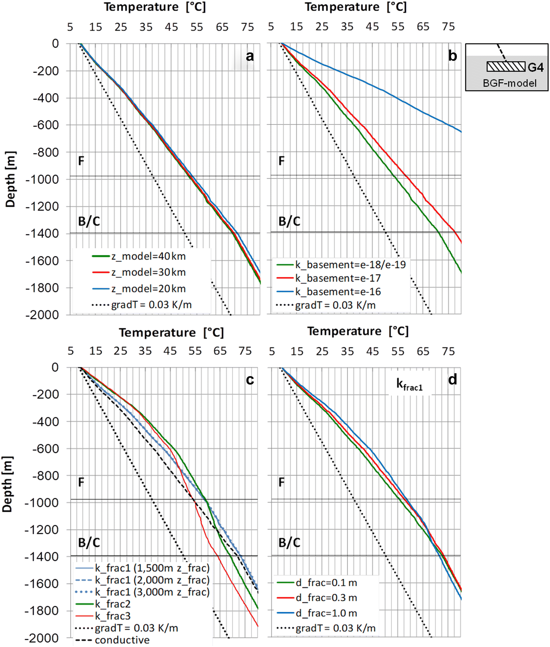
For the sensitivity analysis of the model extension, we chose the BGF-model with the largest granite geometry
G
4 at greatest pluton depth of 6000 m. The incorporated fault has a maximum depth of 2000 m and the lowest fault permeability
kfrac1
(Table
4
). Implications from this scenario are also valid for smaller granite geometries at shallower depths as well as for the conductive model setups. Figure
4
a shows that
zmodel
values of 20, 30 and 40 km result in almost similar temperature curves at the location of the analysed profile
P
(Fig.
3
b). By increasing the
zmodel
values, the modelled temperatures slightly decrease, but only to a negligible extent. For computing time and capacity reasons, we, therefore, uniformly set
zmodel
to 20 km.
Table 4
Variable parameters of the tested model setups and evaluation of the modelled temperature with respect to the measured temperatures in well MueB6
Thermal regime
Model setup (Fig. 3)
BHF (W m−2)
Granite cross-sectional area (Table 3)
kfrac (m2)
Reproduction of T-Log1_MueB6a
Cross-reference
Conductive
B-model
0.070
–
–
No
Figure 6
0.115
–
–
Yes (> 1000 m)
Figure 14
BG-model
0.070
G1, G2, G3
–
No
Figure 10
G4
–
Yes (> 1000 m)
Figure 14
Conductive + convective
BF-model
0.070–0.115
0.070–0.115
0.070–0.105
0.115
–
1 × 10⁻¹²
5 × 10⁻¹³
1 × 10⁻¹³
1 × 10⁻¹³
No
No
No
Yes (< 800 m)
Figure 8
–
Figure 8
Figure 14
BGF-model
0.070
0.070
G2, G3
G4
1 × 10⁻¹³
1 × 10⁻¹³
No
Yes (< 800 m)
Figure 12
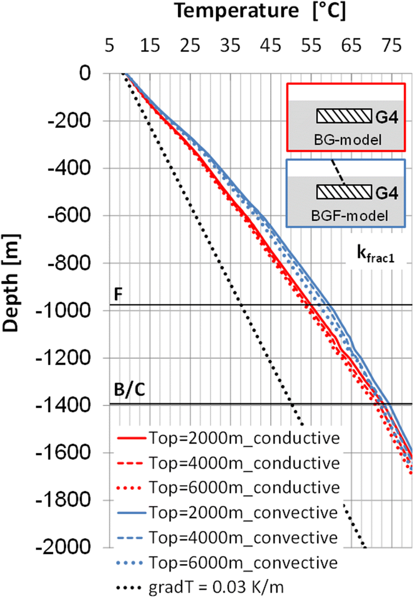
Figure 14
BGF-model modified2)
0.070
G4
1 × 10⁻¹³
Yes
Figure 14
Fig. 4
Sensitivity analysis of
a
the model depth (
zmodel
),
b
the basement permeability (
kbasement
),
c
the fault permeability (
kfrac
) and the maximum depth extent of the implemented fault zone (
zfrac
) and
d
) the width of the implemented fault (
dfrac
) for the permeability value
kfrac1
(BGF-model with granite geometry
G
4 (Table
3
) in 4000 m depth
In order to eliminate the influence of the lateral model extension (
dmodel
), infinite elements were defined as lateral model boundaries (Fig.
3
b), which prevent boundary effects and ensure that the model results are not influenced by the lateral model boundaries (“
Initial and boundary conditions
”). The sensitivity analysis of
dmodel
reveals that tested
dmodel
values of 35, 40 and 50 km result in exactly the same temperature curves (not illustrated). The application of infinite elements eliminates the influence of
dmodel
and, therefore, can be regarded as a very appropriate lateral boundary condition for thermo-hydraulic modelling. For all tested scenarios,
dmodel
was set to 40 km, as the largest granite geometry already has a lateral extension of 30 km and isotherms in the surrounding host rocks can be analysed.
Opening width and permeability of the fault
In a first approach for the convective model setups, we carried out sensitivity analyses for the opening width (
dfrac
) of the implemented fault zone, as well as for its maximum depth (
zfrac
) and permeability (
kfrac
). The effect of these model parameters was also tested with the specific BGF-model setup, used for sensitivity analysis of the model extensions. For sensitivity analysis of
kfrac
, we uniformly set
dfrac
to 0.3 m.
Figure
4
c shows that, compared to the temperature distribution from a solely conductive heat transfer, the three tested permeability values of the fault (
kfrac1
–
kfrac3
) lead to a considerable temperature rise within the sedimentary cover, but with diverging temperature distributions with increasing depth. This implies an enhanced upward convective heat transport via fluid circulation along the fault. The lowest fault permeability
kfrac1
yields a relative continuous temperature rise down to 1600 m depth. In contrast, the higher permeabilities
kfrac2
and
kfrac3
lead to higher temperatures in the upper part of the investigated profile
P
(0–800 m). However, in the lower part (800–1200 m), a considerable decrease of the temperature gradient is observed. This is caused by an enhanced upward heat transport from a lower crustal level due to higher fault permeabilities. Within the area of the sedimentary cover, the thermal profile is convexly upward shaped, resulting from convectional heat transfer in this part of the model (Fig.
4
c). In contrast, the temperature profile of the basement rock layers shows a linear increase in temperatures with depth, resulting from the purely conductive heat transport in this part of the model.
The maximum depth of a fault zone (
zfrac
) might also influence the temperature field, caused by convectional fluid circulation along a permeable fault. Therefore, an additional sensitivity analysis of this parameter was carried out.
zfrac
values of 1500, 2000 and 3000 m were applied in the BGF-model which comprises:
the largest granite
G
4 at 4000 m depth,
a normal BHF of 0.070 W m
−2
,
the lowest tested fault permeability
kfrac1
.
The results of the simulations imply that in our model setup,
zfrac
does not influence the evolving temperature distribution with depth, resulting in equal temperature-depth profiles from varying
zfrac
at the location of the profile
P
(Fig.
4
c). This is also valid for all other scenarios and tested
kfrac
values and implies that the maximum depth extension of a permeable fault into impermeable basement rocks cannot be predicted from the presented model. As all tested
zfrac
scenarios reach the impermeable basement layers (where heat is only transferred by conduction), the long simulation period of 300 Ma always led to similar steady-state conditions at the end of the modelling, independent of the applied
zfrac
value. The isotherms in the area of the fault show steep convex upward shapes (Fig.
5
), typical for convective heat transport [
43
]. A closer look at the temperature distribution in the surrounding of the fault zone reveals that the temperature elevation in the sedimentary cover is restricted to areas very proximal to the fault. The lateral sphere of influence is ~ 500 m and reduces towards the surface (Fig.
5
). The only localised influence of hydraulically active faults on the temperature field has also been postulated for the German Molasse Basin [
66
].
Fig. 5
Isotherms in the area of a 2000 m deep fault after 300 Ma. The fault permeability is set to 10
−13
m
2
(k
frac
1
). The dashed white line indicates the position of the analysed profile
P
(Fig.
3
b). (BGF-model with granite geometry G4 (Table
3
) in 4000 m depth; BHF is set to 0.070 W m
−2
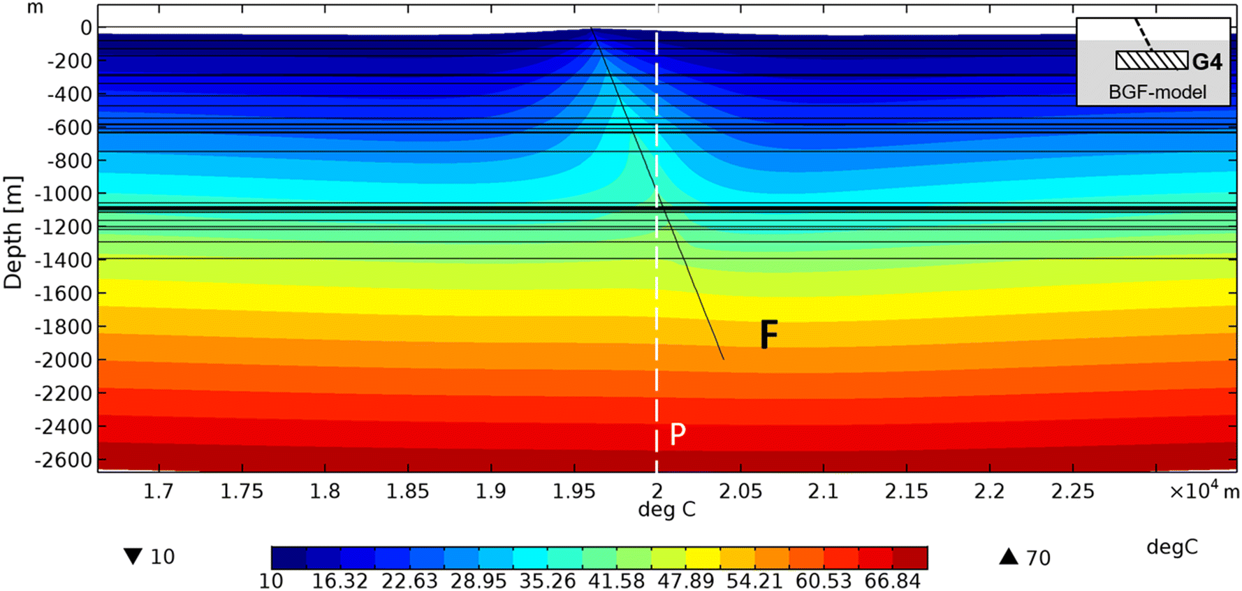
)
The sensitivity analysis for
dfrac
was done with three
dfrac
values: 0.1, 0.3 and 1.0 m.
zfrac
was held constant at 2000 m and the permeability was chosen to be
kfrac1
. Figure
4
d shows that
dfrac
variance considerable influences the evolving temperature distribution with depth. Temperatures in the upper part of the temperature-depth profile increase with increasing
dfrac
, whereas a very high
dfrac
value of 1.0 m leads to lower temperatures below 1400 m, compared to the implementation of smaller
dfrac
values. As subsurface fault geometries and their hydraulic properties usually are not known very well, they mostly have to be estimated for thermo-hydraulic modelling. In this study, we uniformly set
dfrac
to 0.3 m as a larger fracture width is assumed to be unrealistic. However, the high impact on the temperature field of both,
dfrac
and
kfrac
values demonstrate that the hydraulic parameterization of fault zones is a significant source of error in the quantification of temperature distributions in this study and in thermo-hydraulic simulations in general.
Hydraulic properties of the basement rocks
In all model setups the basement rocks were set as impermeable [
65
], allowing only conductive heat transfer in this part of the models. However, any basement permeability may significantly increase the thermal impact of a heat source in the subsurface [
20
,
24
]. In addition, significant basement bulk permeabilities may lead to the formation of deep circulation cells [
67
]. Open fractures have been proven to exist even below 3000 m depth [
49
,
69
]. Fracture permeabilities might be present up to 30 km depth and might cause basement permeabilities even up to 10
−15
m
2
in granites [
62
,
68
].
To verify the impact of the basement rock permeability (
kbasement
) parameter in the model setup presented, a sensitivity analysis of the basement permeability was run for the BGF-model setup, comprising the largest tested granite geometry
G
4 and a 2000 m-deep fault of
kfrac1
.
If
kbasement
is set to ≤ 1 × 10
−18
m
2
, heat is only transferred by conduction in the basement layers. If instead
kbasement
is set to > 1 × 10
−18
m
2
, convection starts and temperatures in the overburden increase significantly (Fig.
4
b). The temperature rise is even more extreme, if
kbasement
is set to 1 × 10
−16
m
2
, indicating a more logarithmic relationship between
kbasement
and the amount of heat transported towards the surface. This is in good agreement with results of other studies, which indicate a threshold permeability of 10
−17
m
2
[
70
] or 10
−16
m
2
[
62
], above which free convection is contributing significantly to the total heat transfer in the upper crust. The temperature distribution is directly affected by the permeability of the host rocks as well as by the permeability of the heat source, i.e. the granitic pluton [
43
].
It is, therefore, concluded that the frequently unknown hydraulic properties of basement rock units provide a major uncertainty factor in thermo-hydraulic parameterization of deep geothermal systems. For example, in our study area neither a high nor a low permeability of the basement rocks can be excluded. Moreover, even if permeable faults are present in the deeper subsurface, hydraulic and thermal gradients would be needed to enable fluid flow.
Model setups without granite
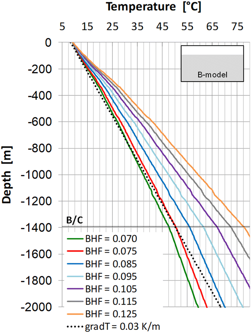
Basic model (B-model): Enhanced BHF in a pure conductive regime
For the scenario of an enhanced BHF acting as heat source at the bottom of the model, we established two model setups:
the basic model (B-model), where only conductive heat transport is allowed and,
the basic model with fault (BF-model), where additional convectional heat transport is allowed along a permeable fault zone and within the pore space of the sedimentary cover (Fig.
3
a).
Both model setups were run with BHF values of 0.070–0.125 W m
−2
. Figure
6
illustrates the resulting temperature–depth profiles for different BHF values in the conductive B-model. The temperature curves for different BHF values imply that they highly impact the temperature distribution in the overburden. At higher BHF values, the temperature in the upper part of the model rises linearly. A BHF of 0.070 W m
−2
results in a temperature distribution expected from a normal continental grad
T
of 30 K km
−1
. An increase in BHF of 10 mW m
−2
then generates about 8% higher temperatures within the sedimentary cover (Fig.
6
).
Fig. 6
Temperature distribution at location of profile
P
in the conductive B-model for BHF values between 0.070 and 0.125 W m
−2
The temperature–depth profiles of the B-model show a linear temperature rise with depth. The temperature log breaks correspond to the thermal conductivity contrasts of the model layers (Table
1
), which is especially obvious at the boundary between the basement rocks and the lower conductive sedimentary cover (Fig.
6
).
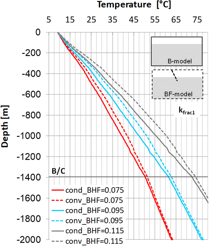
Basic model with fault (BF-model): Enhanced BHF in a convective regime
To test the effect of an enhanced BHF in combination with a deep-reaching permeable fault, the basic model with fault (BF-model) was chosen (Fig.
3
a). In this setup, convection is allowed in the model layers of the sedimentary cover and along the implemented fault zone. The area of the basement rocks is impermeable and only heat conduction is allowed. We run the simulations for both, the lowest and the highest fault permeabilities (
kfrac1
+
kfrac3
). As the maximum depth of the fault does not influence the results of the presented model setup (Fig.
4
c),
zfrac
was uniformly set to 2000 m in all models discussed below.
Compared to the results of the conductive setup of the B-model (Fig.
6
), the presence of a permeable fault (
kfrac1
) and convection within the pore space of the sedimentary cover increase the heat accumulation derived from the deep-seated heat source, in the overburden by about 10% (Fig.
7
).
Fig. 7
Temperature distributions at location of profile
P
for BHF values of 0.075, 0.095 and 0.115 W m
−2
: comparison of the results of the conductive B-model and the convective BF-model (permeability of the fault is set to
kfrac1
)
However, the temperature distribution derived from the BF-model is strongly controlled by
kfrac
. The lowest fault permeability
kfrac1
yields a relative continuous temperature rise with depth. In contrast, the highest fault permeability
kfrac3
leads to significantly higher temperatures in the upper part of the model and causes temperature stagnation in the lower part (800–1200 m), accompanied by significantly lower temperature gradients in this part of the model (Fig.
8
). Nonetheless, regardless of the set
kfrac
, a linear increase in heat source power results in a linear temperature increase in the model (Fig.
8
).
Fig. 8
Temperature distributions at location of profile
P
in the BF-model for BHF values between 0.075 and 0.115 W m
−2
. Fault permeability is set to
kfrac1
and
kfrac3
Model setups with granite
Sensitivity analysis of granite intrusion depth
In a first approach for the model configurations with a heat-producing granite (BG-model + BGF-model, Fig.
3
a), a sensitivity analysis was carried out concerning the influence of the absolute depth level of the pluton on the resulting temperature distribution. As granites are potential targets for geothermal projects [
69
,
71
,
72
], a proper estimation of their depth from thermo-hydraulic simulations would be priceless.
However, Fig.
9
implies that the absolute depth of a heat-producing pluton does not exert a considerable influence on the temperature distribution in the sedimentary cover after 300 Ma. This observation is valid for both tested types of heat transfer. Intrusion depths of 2000, 4000 and 6000 m result in almost similar temperature–depth profiles, with only slightly higher temperatures at shallower intrusion depths of the pluton (Fig.
9
). This is likely related to the fact that the heat source is always situated within the area of the impermeable basement, in which only conductive heat transfer occurs. The time span of the simulation is sufficiently long for reaching similar steady-state conditions independent from the depth position of the pluton. It can be concluded that the absolute depth of a heat-producing pluton—at constant basin configuration and heat production rate—only at shorter simulation times (or younger intrusion ages) would generate a signature in the temperature field.
Fig. 9
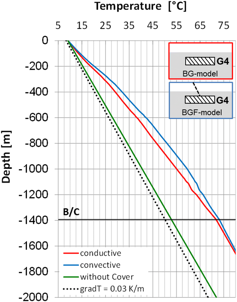
Sensitivity analysis of the variation of the pluton top depth level in the BG-model and BGF-model
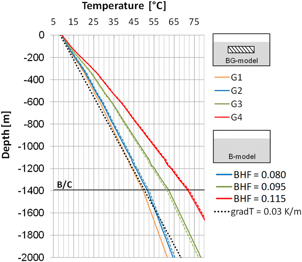
Basic model with granite (BG-model): various dimensions of heat-producing granites in a conductive regime
In the conductive basic model with granite (BG-model), we tested four geometries of moderately heat-producing granites, which have various cross-sectional areas of 11.55–300 km
2
(Table
3
). As the depth of the pluton top does not significantly influence the temperature distribution after 300 Ma (Fig.
9
), we uniformly set the granite top at 4000 m depth. For all tested underground scenarios with granite, the BHT at the bottom of the model was set to 0.070 W m
−2
and
Agranite
is set 6 μW/m
3
(Table
4
).
By applying pure conduction (BG-model), the small granite volumes
G
1 and
G
2 with cross-sectional areas of 11.55 and 35.0 km
2
only cause a small temperature rise in the overburden, compared to the temperature profile of a normal continental grad
T
(Fig.
10
). In contrast, the larger granites
G
3 and
G
4 lead to considerably higher temperatures in the upper part of the model. Figure
10
also suggests that the thermal impact of a heat-producing pluton linearly increases with increasing volume.
Fig. 10
Comparison of the temperature distribution at the location of profile
P
for (1) the four tested pluton geometries (Table
3
) in the BG-model and (2) varying BHF values of 0.080, 0.095 and 0.115 W m
−2
as only heat source in the B-model
A granite geometry
G
2 (BG-model) and a slightly enhanced BHF of 0.080 W m
−2
(B-model) cause a similar temperature rise in the sedimentary cover (Fig.
10
). The temperature effects of the granites
G
3 and
G
4 (BG-model) are comparable to the heat supply by a BHF of 0.095 W m
−2
and 0.115 W m
−2
(B-model), respectively (Fig.
10
).
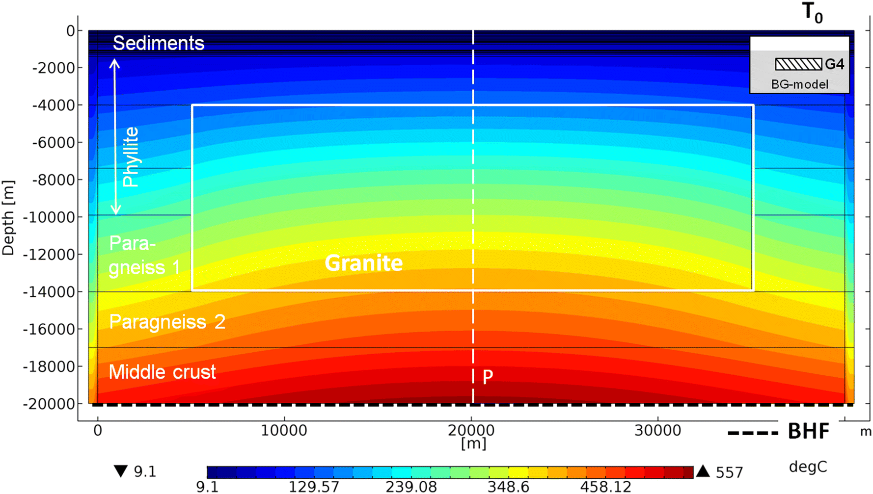
Figure
11
illustrates the isotherms of the BG-model applying granite geometry
G
4 at 4000 m depth after 300 Ma forward modelling. The heat production of the granite induces a temperature rise below and above the pluton, with its maximum in the central part of the heat source. The isotherms have a broad convex upward shape, which rapidly flattens with increasing distance to the heat source, considered typical for purely conductive cooling [
43
].
Fig. 11
Isotherms in the BG-model with pluton geometry
G
4 in 4000 m depth after 300 Ma. The dashed white line indicates the position of the analysed profile
P
(Fig.
3
b). The BHF is set to 0.070 W m
−2
and
Agranite
is 6 μW m
−3
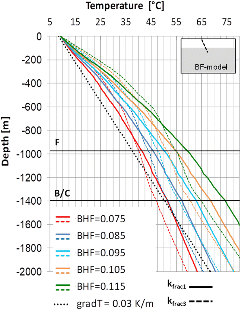
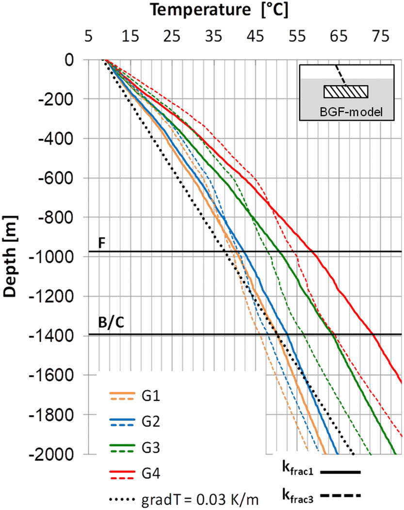
Basic model with granite and fault (BGF-model): Various sizes of heat-producing granites in a convective thermal regime
In the BGF-model setup, we tested the effect of additional convective heat transport in the granite model. The simulations were run for the fault permeabilities
kfrac1
and
kfrac3
.
Compared to the conductive granite model setup (BG-model; Fig.
10
), the granitic heat-source has a higher thermal impact on the overburden, if convection is allowed (Fig.
12
). The effects of different
kfrac
values are independent of the heat source in the model. As already demonstrated in Fig.
8
, the higher fault permeability
kfrac3
leads to an elevated temperature in the upper part of the model, accompanied by a flatter grad
T
in the lower part of the sedimentary cover. The significantly lower
kfrac1
value causes a more continuous temperature rise with depth.
Fig. 12
Temperature distributions at location of profile
P
from granite geometries
G
1–
G
4 in the BGF-model. Fault permeability is set to
kfrac1
and
kfrac3
The temperature field is furthermore controlled by the size of the granite, independent of whether conductive or convective heat transport is considered (Figs.
10
,
12
). The thermal impact of a deep-seated heat-producing pluton linearly increases with its volume. The simulations confirm that any convectional component generally increases the efficiency of heat transport from the heat source [
24
]. However, elevated temperatures due to fluid circulation on a hydraulically active fault zone are limited to areas very proximal to the fault (Fig.
5
).
The insulation effect of a low conductive sedimentary cover
Another factor contributing to the formation of local temperature anomalies in sedimentary basins might be the presence of thick, low conductive sedimentary rock layers above a heat source. As thermal conductivity exerts a first-order control on the temperature field in the underground [
24
], a significant effect on the resulting temperature distribution in the model can be expected by the variation of this parameter. Low conductivity rocks potentially act as insulators below which heat can be accumulated, resulting in high-temperature gradients (e.g., [
51
,
73
,
74
], also at economically relevant depths < 5 km [
51
].
To investigate the effect of missing sediment cover with rock layers of low thermal conductivity (e.g., clay- and marlstones) in the modelled part of the sedimentary basin, the thermal conductivity contrast between the sedimentary cover (mean: 2.8 W m
−1
K
−1
) and the basement (phyllite: 3.7 W m
−1
K
−1
) was removed. In the BG- and BGF-model setups, the thermo-hydraulic properties of the sedimentary layers were replaced by the input parameters of the uppermost phyllitic basement rock layer (Table
1
). The removal of the thermal conductivity contrast results in a temperature–depth profile (green curve) that provides only slightly higher temperatures than the temperature distribution generated by a normal continental grad
T
(Fig.
13
). The absence of an insulating sedimentary cover prohibits the accumulation of heat generated by the heat-producing granite. This demonstrates the important role of a low-conductive, insulating blanket for the emergence of temperature anomalies in sedimentary basins, charged by any deep-seated heat source. Moreover, the effect of decreasing thermal conductivities with increasing temperatures at depth can even reinforce the insulating effect of a sedimentary cover [
75
].
Fig. 13
Test of the insulation effect of the sedimentary cover: comparison of the temperature distribution at the location of profile
P
in the BG-model and BGF-model, when (1) the measured thermal conductivities of the sedimentary cover are used, or (2) the thermal conductivity of the sedimentary cover is uniformly set to the basement rock conductivity of the phyllites 3.7 W m
−1
K
−1
(Table
1
)
The extreme effect of variable thermal conductivity of the sedimentary cover layers in the models presented confirms that this parameter is a first-order control factor for the temperature distribution in the subsurface [
24
]. This in turn points out that for valid thermo-hydraulic models, a careful parameterization of the thermal properties of the subsurface lithologies in the target area is essential. The acquisition of statistically valid thermo-hydraulic data by extensive measurement campaigns, therefore, is essential, if there is no local data pool available from the target area.
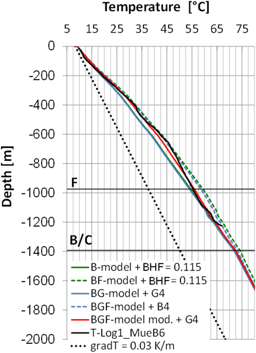
Implications for the temperature anomaly in the Franconian Basin
Our models allow a first evaluation of the impact of the tested heat sources and geological conditions in generating the Franconian Basin (Mürsbach) temperature anomaly in SE Germany. Because the extrapolation of temperature logs generally bears considerable uncertainty, the modelled thermal profiles are only discussed down to the final depth of
T
-Log1_MueB6 at 1204.2 m, as the input data of this model section are based on measured data.
The modelled temperature distributions imply that an average BHF (generating a normal continental grad
T
in the conductive B-model, Fig.
6
), is not sufficient for achieving the measured temperatures in the case study area for both tested assumptions—a solely conductive or combined conductive/convective heat transport (Fig.
13
). However, there are several potential scenarios for achieving the elevated temperatures observed in the
T
-Log1_MueB6. By assuming a purely conductive regime, measured temperatures below 1000 m depth are reproduced by the following:
an elevated BHF of 0.115 W m
−2
or
the presence of a heat-producing granite of large size (
G
4) and a heat production rate of 6 μW m
−3
, combined with an average BHF of 0.070 W m
−2
at the bottom of the model (Fig.
14
, Table
4
).
Fig. 14
Comparison of the measured temperature log in well MueB6 and the modelled temperature profiles from (1) the B-model and BF-model, each with BHF = 0.115 W m
−2
, (2) BG-model and BGF-model, each with granite geometry G4, and (3) a modified BGF-model, allowing conductive heat transfer only in the Permian rock units below 1059 m (Table
1
)
However, the measured temperatures in the Triassic section of the well at 300–1000 m depth (Table
1
) could not be reproduced by a purely heat conductive scenario. In this section, the temperature log of well MueB6 is rather convex upward, pointing to a convective heat transport component. The measured temperatures were reached applying additional heat transport along a fault of
kfrac1
for both scenarios described above (Fig.
14
, Table
3
). The temperature curves from fault permeability
kfrac1
in combination with a THF of 0.115 W m
−2
reproduce the log section between at 300 and 1000 m depth. Similar results are achieved by the BGF-model with granite geometry
G
4. However, modelled temperatures derived from these scenarios are slightly too high in the well section below 1000 m. This suggests that below 1000 m (Zechstein section; Table
1
), heat may predominantly be transferred by conduction, whereas in the upper part of the sedimentary cover also convection seems to play a key role in heat transport. This assumption is confirmed by the modelled temperature profile of a modified BGF-model setup with granite geometry
G
4 (BGF-model mod.), where only conduction is allowed in the Permian section of well MueB6 (Fig.
14
). Such a scenario provides the best reproduction of the measured temperature log, including the 900–1200 m section.
Thus, an elevated BHF in combination with a permeable fault zone of
kfrac1
or the scenario of a heat-producing granite of cross-sectional area
G
4 in combination with an average BHF of 0.070 W m
−2
would provide the best explanations for the elevated temperatures in the case study area (Table
4
). A purely conductive regime in the centre of the investigated temperature anomaly can be excluded, as the measured temperature log cannot be completely reproduced by the purely conductive scenarios tested. Similar conclusions have been drawn in a study of the North Alpine Foreland Molasse Basin, where heat transport in the deeper part is mainly conductive, but strongly influenced by fluid flow within the overlying sediment fill [
66
].
However, preliminary results of gravity modelling [
53
] do not indicate the presence of such a large granite volume in the deeper underground of the well MueB6 location. Therefore, convective heat flow along hydraulically active faults and/or an elevated BHF might provide a more realistic explanation for the local high temperature. As the presence of deep reaching faults is known from local seismic surveys, a key prerequisite for convective heat transport exists. However, a permeable fault alone without additional heat source—may it be an enhanced BHF, a heat-producing granite, a combination of both or other sources—is not sufficient for achieving the measured temperature profiles.
Implications and outlook for future geothermal exploration in the Franconian Basin
The presented conceptual 2-D models show that the thermo-hydraulic parameterization of the implemented fault zone, the basement layers and the sedimentary cover has a very high impact on temperature distributions resulting from thermo-hydraulic simulations. In addition, the volumes and heat production rates of the heat sources tested highly affect the evolving temperature field. With regard to a future geothermal exploration in the Franconian Basin, the lacking knowledge of the structure of the deeper subsurface as well as of the hydraulic properties of fault zones is a major data gap, which must be closed by further research. Currently, an extensive seismic survey program is being conducted in the Franconian Basin aiming to get more detailed information on the basement topography and the structural framework of the deeper subsurface [
76
].
Relatively simple, conceptual models, as the one presented here, are a valuable tool for the early stage exploration of geothermal reservoirs. For example, they can be used as plausibility tests for the evaluation of the thermal impact of specific heat sources and of the thermo-hydraulic boundary conditions, which are suspected as causing thermal anomalies in comparable geological settings. This is in particular true when dealing with small data sets at different scales. Herein, our model setup can be used as a first approach to verify hypotheses of specific underground scenarios which then can be further developed for a more complex 3-D simulation. They may also be used for an initial assessment, whether the volume of a heat-producing granite would be large enough to provide detectable signatures, e.g. in gravity modelling.
Conclusions
This study presents 2-D thermo-hydraulic simulations of a conceptual geothermal system, comprised of a deep-seated heat source within impermeable basement, covered by low conductive sediments. The test of two different heat sources, namely a heat-producing granite and different values of background heat flow (mainly generated by radioactive decay in the mantle and the crust), demonstrate that the resulting temperature distribution is strongly controlled by the following:
the volume of the heat-producing granite,
the amount of the background heat flow,
the permeability of the basement rocks hosting the heat source,
the insulating effect of a low thermal conductivity cover above the heat source,
the permeability of hydraulically active faults, and
the predominant heat transfer process (conduction vs convection).
Any heat source is provided a much higher heat transport efficiency from deeper parts of the crust upward in the case of combined conductive and convective heat transport components.
Sensitivity analysis reveals that major uncertainties for reliable temperature distributions in the simulated geothermal system arise from the hydraulic parameterization of implemented fault zones and of basement layers. Changes in permeability values have a strong influence on the effectivity of the heat source and on the resulting temperature field. In the model, the removal of thermal conductivity contrasts between the basement layers and the sedimentary cover had a negative effect on the heat accumulation within the sediments above the heat source. This demonstrates the need of an insulating, low thermal conductivity sedimentary blanket, as a prerequisite for the emergence of this type of thermal anomaly. The first-order control of thermal conductivity values also illustrates the importance of a careful parameterization of the thermal properties of the subsurface lithologies in the target area. If there is no regional data pool already available, the acquisition of statistically valid thermo-hydraulic data by extensive measurement campaigns is, therefore, considered as an essential prerequisite in geothermal exploration.
The models presented here were calibrated on structural and thermo-hydraulic data of the Franconian Basin in SE Germany. Therefore, the results also allow the evaluation of different hypotheses for the structure of the subsurface, which are treated as potential cause of the temperature anomaly investigated. An equilibrium temperature log measurement could only be reproduced by the following:
an enhanced background heat flow of 0.115 W m
−2
in combination with a permeable fault zone of permeability 1.0 × 10
−13
m
2
or
a heat-producing granite of very large cross-sectional area (300 km
2
) in combination with an average background heat flow of 0.070 W m
−2
.
Although new 2D seismic surveys are in progress, there is no convincing evidence from existing gravity data for the existence of such a voluminous granite body beneath the centre of the examined temperature anomaly. Tentatively, we, therefore, prefer the first of the two latter scenarios. In addition, a purely conductive regime in the study area can be excluded, as the temperature-depth profile of the measured log cannot be completely reproduced by the conductive scenarios tested.
Our conceptual 2-D models can provide first proxies and plausibility tests for the evaluation of the thermal impact of specific heat sources and of the thermo-hydraulic boundary conditions, which are suspected as causing thermal anomalies in comparable geological settings. They may also be used for an initial assessment, whether the volume of a heat-producing granite would be large enough to provide detectable signatures, e.g. in gravity modelling.
Acknowledgements
We thank our collaborators of the Bayerisches Landesamt für Umwelt (LfU) for providing core material as well as thermal conductivity data of the basement rocks (well Obernsees 1). We thank Prof. Helga de Wall for scientific advice and financial support for the procurement of the modelling software. Thanks also to Dr. Michael Drews, Dr. Hagen Deckert and Dr. Wolfgang Bauer for scientific support.
Publisher's Note
Springer Nature remains neutral with regard to jurisdictional claims in published maps and institutional affiliations.
References
Gudden (1981) Über Thermal-Mineralwasser-Bohrungen im Coburger Umland (pp. 229-252)
Unknown ()
Unknown ()
Stober and Bucher (2013) Springer
Rybach et al. (2018) Geothermal energy and a future earth Cambridge University Press 10.1017/9781316761489.035
Cěrmák and Bodri (1995) Three-dimensional deep temperature modelling along the European geotraverse10.1016/0040-1951(94)00214-T
Sandiford and Powell (1986) Deep crustal metamorphism during continental extension: modern and ancient examples10.1016/0012-821X(86)90048-8
Waples (2001) A new model for heat flow in extensional basins: Radiogenic heat, asthenospheric heat, and the McKenzie Model10.1023/A:1012521309181
Hecht (1993) Die geothermischen Verhältnisse in der Bohrung Bad Colberg 1/1974 (pp. 121-128)
Hicks et al. (1996) A Hydro-thermo-mechanical numerical model for HDR geothermal reservoir10.1016/0148-9062(96)00002-2
Nabelek et al. (2001) Thermo-rheological, shear heating model for leucogranite generation, metamorphism, and deformation during the Proterozoic Trans-Hudson orogeny, Black Hills, South Dakota10.1016/S0040-1951(01)00171-8
Kukkonen and Lauri (2009) Modelling the thermal evolution of a collisional Precambrian orogen: high heat production migmatitic granites of southern Finland10.1016/j.precamres.2008.10.004
Kim and Lindquist (2003) Fracture flow simulation using a finite-difference lattice Boltzmann method10.1103/PhysRevE.67.046708
Nabelek et al. (2012) The influence of temperature-dependent thermal diffusivity on the conductive cooling rates of plutons and temperature-time paths in contact aureoles10.1016/j.epsl.2011.11.009
Dietl and Longo (2007) Thermal aureole around the Joshua Flat-Beer Creek Pluton (California) requires multiple magma pulses: constrains from thermobarometry, infra-red spectroscopy and numerical modelling10.1127/1864-5658/07/0095-0013
Kosakowski et al. (1999) Hydrothermal transients in Variscan crust: paleo-temperature mapping and hydrothermal models10.1016/S0040-1951(99)00064-5
Casini (2012) A MATLAB-derived software (geothermMOD1.2) for one-dimensional thermal modeling, and its application to the Corsica-Sardinia batholith10.1016/j.cageo.2011.10.020
Freudenberger and Schwerd (1996) Bayerisches Geologisches Landesamt
Schäfer et al. (2000) Upper-plate deformation during collisional orogeny: a case study from the German Variscides (Saxo-Thuringian Zone)10.1144/GSL.SP.2000.179.01.17
Unknown ()
Finger et al. (1997) Variscan granitoids of central Europe: their typology, potential sources and tectonothermal relations10.1007/BF01172478
Blecha and Štemprok (2012) Petrophysical and geochemical characteristics of late Variscan granites in the Karlovy Vary Massif (Czech Republic)—implications for gravity and magnetic interpretation at shallow depth10.3190/jgeosci.115
Abratis et al. (2007) Two distinct Miocene age ranges of basaltic rocks from the Rhön and Heldburg areas (Germany) based on 40Ar/39Ar step heating data10.1016/j.chemer.2006.03.003
Peterek et al. (1996) Neogene Tektonik und Reliefentwicklung des nördlichen KTB-Umfeldes (Fichtelgebirge und Steinwald) (pp. 7-25)
Peterek et al. (1997) The late- and post-Variscan tectonic evolution of the Western Border fault zone of the Bohemian massif (WBZ) (pp. 191-202) 10.1007/s005310050131
Unknown ()
Unknown ()
Heidbach et al. (2016) WSM team: world stress map database release 201610.5880/WSM.2016.001
Förster (2001) Analysis of borehole temperature data in the northeast German Basin: continuous logs versus bottom-hole temperatures 7(3) (pp. 241-254) 10.1144/petgeo.7.3.241
Rider and Kennedy (2011) Rider-French Consulting
Popov et al. (1999) Characterization of rock thermal conductivity by high-resolution optical scanning (pp. 253-276) 10.1016/S0375-6505(99)00007-3
Filomena et al. (2014) Assessing accuracy of gas-driven permeability measurements: a comparative study of diverse Hassler-cell and probe permeameter devices10.5194/se-5-1-2014
Zimmerman (2006) World Scientific Pub. 10.1142/6141
Norton and Knight (1977) Transport phenomena in hydrothermal systems: cooling plutons10.2475/ajs.277.8.937
Unknown ()
Stettner and Salger (1985) Das Schiefergebirge in der Forschungsbohrung Obernsees (pp. 49-55)
de Wall et al. (2019) Subsurface granites in the Franconian Basin as the source of enhanced geothermal gradients: a key study from gravity and thermal modeling of the Bayreuth Granite10.1007/s00531-019-01740-8
Cherubini et al. (2013) Impact of single inclined faults on the fluid flow and heat transport: results from 3-D finite element simulations10.1007/s12665-012-2212-z
Somerton (1992) Elsevier
Clauser et al. (1997) The thermal regime of the crystalline continental crust: implications from the KTB10.1029/96JB03443
Abdulagatov et al. (2006) Effect of pressure and temperature on the thermal conductivity of rocks10.1021/je050016a
Unknown ()
Scharfenberg et al. (2016) In situ gamma radiation measurements on Variscan granites and inferred radiogenic heat production, Fichtelgebirge, Germany10.1127/zdgg/2016/0051
Siebel et al. (2010) Permo-Carboniferous magmatism in the Fichtelgebirge: dating the youngest intrusive pulse by U–Pb, 207Pb/206Pb and 40Ar/39Ar geochronology 38(2/3) (pp. 85-98)
Förster et al. (2008) Chemical composition of radioactive accessory minerals: implications for the evolution, alteration age, and uranium fertility of the Fichtelgebirge granites (NE Bavaria, Germany)10.1144/petgeo.7.3.241
Parsons (1966) Permeability of idealized fractured rock10.2118/1289-PA
Snow (1968) Rock fracture spacings, openings, and porosities 94(1) (pp. 73-92)
Oda (1986) An equivalent continuum model for coupled stress and fluid flow analysis in jointed rock masses10.1029/WR022i013p01845
Norton and Knapp (1977) Transport phenomena in hydrothermal systems: the nature of rock porosity10.2475/ajs.277.8.913
Unknown ()
Unknown ()
Cherubini et al. (2014) Influence of major fault zones on 3-D coupled fluid and heat transport for the Brandenburg region (NE German Basin)10.5194/gtes-2-1-2014
Przybycin et al. (2017) The origin of deep geothermal anomalies in the German Molasse Basin: results from 3D numerical models of coupled fluid flow and heat transport10.1186/s40517-016-0059-3
Jobmann and Clauser (1994) Heat advection versus conduction at the KTB: possible reasons for vertical variations in heat-flow density10.1111/j.1365-246X.1994.tb00912.x
Unknown ()
Unknown ()
Blackwell et al. (1989) Thermal conductivity of sedimentary rocks: measurement and significance Springer 10.1007/978-1-4612-3492-0_2
Meixner et al. (2014) Using constrained gravity inversions to identify high-heat-producing granites beneath thick sedimentary cover in the Cooper Basin region of central Australia10.1016/j.geothermics.2013.10.010
Lemenager et al. (2018) The effect of temperature-dependet thermal conductivity on the geothermal structure of the Sydney Basin10.1186/s40517-018-0092-5
Drews et al. (2019) Ursachenforschung zur geothermischen Anomalie in Nordbayern (pp. 10-13)
Unknown ()
Unknown ()
Unknown ()
Unknown ()
Unknown ()
Unknown ()
Unknown ()
Unknown ()
Freudenberger et al. (1996) Gesteinsfolge des Deckgebirges nördlich der Donau und im Molasseuntergrund Bayerisches Geologisches Landesamt
Burkhardt et al. (1989) Geothermal investigations in the KTB locations Oberpfalz and Schwarzwald (pp. 433-480) Springer 10.1007/978-3-642-74588-1_18
Unknown ()
Unknown ()
Agemar et al. (2014) The geothermal information system for Germany—GeotIS (pp. 129-144)
Hecht (1996) Heilbäder Südthüringens aus balneologischer Sicht (pp. 173-191)
Hecht (1999) Die geologischen Ergebnisse der Thermalsolebohrung Bad Colberg 1994 (pp. 29-49)
Trusheim (1964) Über den Untergrund Frankens: Ergebnisse von Tiefbohrungen in Franken und Nachbargebieten 1953–1960 (pp. 1-11)
Unknown ()
Birzer (1956) Die Mineralwasserbrunnen von Fürth in Bayern (pp. 106-118)
von Freyberg (1954) Die Randfazies des Gipskeupers, insbesondere der Benker Sandstein in Franken (pp. 3-47)
Unknown ()
Unknown ()
Schmitt (1982) Die Mineralwasserbohrung von Bad Königshofen im Grabfeld mit dem Kurzprofil einer neuen Tiefbohrung (pp. 187-193)
Gudden and Schmid (1985) Die Forschungsbohrung Obernsees—Konzeption, Durchführung und Untersuchung der Metallführung (pp. 5-21)
Unknown ()
Wrobel (1992) Die Thermalwassererschließungsbohrung Rodach 2/1988 (pp. 3-35)
Unknown ()
Unknown ()
Dill (1990) Die Schwermineral-Führung im Permokarbon zwischen Weiden und Schmidgaden. Ein Beitrag zur stratigraphischen Untergliederung des Jungpaläozoikums am Westrand der Böhmischen Masse (pp. 43-59)
Unknown ()
Röckel and Stober (2017) Die neue Tiefbohrung Weißenstadt im Granit des Fichtelgebirges10.1007/s00767-017-0361-4
Unknown ()
Kestin et al. (1978) Viscosity of liquid water in the range − 8 °C to 150 °C10.1063/1.555581
Haywood (1966) Sixth international conference on the properties of steam—supplement on transport properties10.1115/1.3678480
Wooding (1957) Steady state free thermal convection of liquid in a saturated permeable medium10.1017/S0022112057000129
Yusa and Oishi (1989) Theoretical study of two-phase flow through porous medium (II)—occurence of two-phase flow system inferred from analysis of one-dimensional (vertical) steady state model in the case of no net fluid transport10.11367/grsj1979.8.277