Modeling works which simulate the proton-exchange membrane fuel cell with the computational fluid dynamics approach involve the simultaneous solution of multiple, interconnected physics equations for fluid flows, heat transport, electrochemical reactions, and both protonic and electronic conduction. Modeling efforts vary by how they treat the physics within and adjacent to the membrane-electrode assembly (MEA). Certain approaches treat the MEA not as part of the computational domain, but rather an interface connecting the anode and cathode computational domains. These approaches may lack the ability to consistently model catalyst layer losses and MEA ohmic resistance. This work presents an upgraded interface formulation where coupled water, heat, and current transport behaviors of the MEA are modeled analytically. Improving upon the previous work, catalyst layer losses can now be modeled accurately without ad-hoc selection of model kinetic parameters. Key to the formulation is the incorporation of water absorption/desorption resistances. The interface model is developed with the consideration of only thru-plane variation, based upon varied fundamental research into each of the relevant physics. The model is validated against differential cell data with high- and low-humidity reactants. The agreement is very good in each case.

Model development

The MEA is represented as a two-dimensional interface that separates the anode and cathode computational domains. The MEA computational routine accesses the solution variables at the surface of each domain and produces fluxes into each of the physics. The role of the interface model in multi-domain approaches has been to approximate all the externally relevant behavior of the MEA (i.e., current generation, reactant consumption, water permeation, heat generation, etc.) by boundary conditions on both sides of the interface [ ⁶ ].

Model schematic and operation

Figure ² shows an MEA schematic with typical thickness dimensions included. The anode contains hydrogen, water vapor, and inert nitrogen species, while the cathode is modeled as a mixture of oxygen, water vapor, and inert nitrogen. The interface takes as boundary values, the anode (A) and cathode (C) solution variables from the GDL. The interface replaces the MEA, containing the anode catalyst layer (ACL), membrane (MEM) and cathode catalyst layer (CCL) regions, in the center portion of the figure, with sources, acting as boundary conditions.

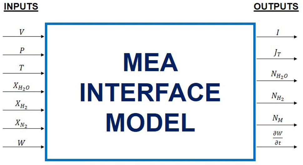
The MEA model has inputs and outputs shown in Fig. ³ . Inputs include gas pressure, temperature, mole fractions, and voltage from the adjacent anode and cathode cells within the gas diffusion layer (GDL). Mole fractions of the species present, such as water, hydrogen, and oxygen, are used similarly to the previous works. The outputs include estimates of current density, heat sources, reactant fluxes, water fluxes, and the water gain rate of the ionomer phase of the MEA.

Inputs and outputs of MEA interface model

MEA composition/description

A description of MEA dimensions and compositions is needed to estimate the various catalyst layer losses. The MEA has three regions: the anode catalyst layer, membrane, and cathode catalyst layer, denoted by ACL, MEM, and CCL, respectively.

The membrane is assumed to be Nafion, a solid ionomer which is nearly impervious to gas penetration, except for water vapor. A constant, selectable equivalent weight EW (g/equiv or g/mol SO ₃ ⁻ ), and density ρIo (g/cm ³ ), is contemplated. Absorbed water with density ρW (g/cm ³ ) exists within the ionomer. A constant crossover current density, Ix (A/m ² ) is assumed: typically, 0.5–1 mA/cm ² (5–10 A/m ² ), as a result of slight hydrogen gas permeation through the membrane from anode to cathode.

The thicknesses of the three MEA zones, denoted tACL , tCCL , and tMEM (m), refer to the dry values; prior to water uptake. Nominal membrane thicknesses refer to values at about 50% RH; hence, a 22 μm-thick dry membrane swells to a 25 μm nominal thickness [ ⁷ ].

PEMFC catalyst layers are porous electrodes: with mixtures of platinum catalyst nanoparticles, the carbon support, the ionomer binder, water sorbed within the ionomer, and void space, that allow for reactant gas diffusion. The ionomer is the same EW as the membrane. The material components, their respective functions within the catalyst layer(s), and their transport roles are summarized in Table ¹ . To define catalyst layer composition, several densities, molecular weights, and fundamental physical constants are listed in Table ² . Catalyst layer composition described in Table ³ is assumed to be spatially uniform throughout its thickness. The composition of the anode catalyst layer (ACL) and cathode catalyst layer (CCL) is determined by four parameters: the platinum loading LACL,Pt (~ 0.1–0.4 mg _Pt cm ⁻² ), the weight percent Pt/carbon in the catalyst powder PtcACL (~ 20–60%), the ionomer-to-carbon ratio ICACL (~ 0.5–1.5) which is the mass ratio of dry ionomer to carbon within the respective catalyst layer, and its thickness tACL (~ 2–12 μm). Once these are known, the composition of the catalyst layer is further described.

Table 1

Material components of catalyst layers

Material component	Function	Transport role
(Pt) Pt nanoparticles	Catalyst particles	Reaction (rxn) site location
(C) Carbon black	Support	e− conduction to rxn site
(Io) Ionomer (typ. Nafion)	Binder	H+ conduction to rxn site
(W) Sorbed water within ionomer	Enhances conductivity of ionomer	H+ conduction to rxn site
(V) Void space	Allows gaseous reactant access	Gaseous reactant transport to rxn

Table 2

Densities and molar masses of catalyst layer components

Densities		(g cm⁻³)	Molar masses		(g mole⁻¹)
ρw	Water density	1.0	MW	Water molar mass	18
ρIo	Ionomer dry density	2.0	EW	Ionomer eq. weight	800–1200 (typ)
ρC	Carbon black density	2.2	MH2	Hydrogen molar mass	2
ρPt	Platinum density	21.0	MO2	Oxygen molar mass	32

Table 3

Catalyst layer and membrane compositions

Catalyst layers		Membrane
tACL	Catalyst layer thickness (m)	tMEM	Membrane thickness (m)
LACL,Pt	Platinum loading mg_Pt cm⁻²	EW	Ionomer equivalent weights (g/mol)
PtcACL	Weight percent Pt/carbon in the catalyst powder (%)	Ix	Crossover current density (A/m²)
ICACL	Ionomer-to-carbon ratio (–)

Derived catalyst layer volume fractions/compositions
εACL,C=LACL,CρCtACL	LACL,C=100-PtcACLPtcACLLACL,Pt
εACL,Io=LACL,IoρIotACL	LACL,Io=LACL,CICACL
εACL,V=1-LACL,Pt/ρPt+LACL,C/ρC+LACL,Io/ρIotACL

Ionomer water uptake

Ionomer equilibrium water uptake is expressed in the form of a non-dimensional water uptake λeq (mol H ₂ O/mol SO ₃ ⁻ ) the number of water molecules per acid site within the ionomer, which normalizes water uptake for any equivalent weight. Uptake from humidity and ionomer swelling with water uptake is described.

Ionomer water uptake is modeled with reference to water activity, or gas humidity, at anode ( αA ) and cathode ( αC ) side adjacent cells using ideal gas mixture relationships. Relative humidity is calculated as in Eq. ( ¹ ), where water vapor saturation pressure PSAT(T) is defined by a fit in Eq. ( ² ) with temperature (K) recommended by [ ⁸ ]. Equilibrium water uptake is curve-fitted from the experimental measurements of Jalani et al. [ ⁹ , ¹⁰ ] with fifth-order polynomials. Uptake from Nafion membranes in contact with liquid water has been observed at λeq=22 water molecules per acid site, while uptake from the vapor phase ranges from λeq=1-2 (10% RH) to λeq=14-16 (100% RH). Water uptake from the liquid phase (300% RH) is λeq=22 , in agreement with several previous authors [ ¹¹ , ¹² ]. Detailed derivation can be found in Edwards [ ¹³ ]:

αA=XH2O,APAPSAT(TA)αC=XH2O,CPCPSAT(TC),

PSAT(T)=2846.4+411.24(T-273.15)-10.554(T-273.15)2+0.16636(T-273.15)3.

Water uptake within the ionomer λ will vary from the equilibrium values λeq . The ionomer is considered a mixture of the two phases: dry membrane and water. The concentration of dissolved water in the ionomer, cW (mol H ₂ O m ⁻³ ), is related to the dimensionless water content λ expressed as in Eq. ( ³ ), where cf is the concentration of fixed charge sites (mol SO ₃ ⁻ m ⁻³ ). The volume fraction of water within the ionomer phase, fV , is given as Eq. ( ⁴ ), where VW represents the molar volume of water (m ³ mol ⁻¹ ) and VIo the molar volume of the ionomer. The corresponding fractional increase in volume of the hydrated ionomer phase, εdV , compared to the dry volume, is in Eq. ( ⁵ ):

cW=cfλ=ρIoEWλ,

fv=λVWVIo+λVW=λMW/ρWEW/ρIo+λMW/ρW,

εdV=VWVIoλ=MWρIoEWρWλ.

Ionomer volumetric swelling results in increased MEA thickness. While the in situ PEMFC environment compresses the MEA, a focused study concluded that, at typical cell assembly pressures, the water uptake is not significantly decreased [ ¹⁴ ]. The swollen membrane thickness with water uptake λ is given in Eq. ( ⁶ ), similar to the experimental kinetics investigations of Liu et al. [ ⁷ ]. Though not as obvious, those investigations contemplate a similar expansion in catalyst layer thickness:

tMEMS=tMEM1+εdV=tMEM1+MWρIoEWρWλ.

Ionomer-phase water/ion transport

The membrane is modeled as impermeable to gases, but considers the absorption, desorption, and permeation of water. The current density J→Io (A m ⁻² ) represents protons (H+) moving through the membrane under the influence of the gradient of the electric potential field of the ionic phase ΦIo . Consumption of hydrogen and oxygen reactants is accounted for by boundary fluxes. Water and current transport within the membrane are assumed to occur only in the thru-plane direction and are treated with the common, de-facto standard phenomenological approach originated by Springer et al. [ ¹⁵ ], using only macroscopic calculations. The flux forms are shown in Eq. ( ⁷ ). When restricted to the thru-plane direction, current density J→Io=I must be constant through the thickness of the membrane:

J→W=ndJ→IoF-cfDW∇λJ→Io=-σIo∇ΦIo.

The three transport properties nd , DW , and σIo exhibit water content and temperature dependence. Property variation makes this problem inherently non-linear and the degree of property variation with changes in water content was said to be substantial [ ¹⁶ ].

The electroosmotic drag coefficient, nd (–), represents the number of water molecules dragged from anode to cathode along with each migrating proton. Typical approximate values have been reported as 0.6–1.0 for vapor-equilibrated membranes and 2–2.5 for liquid-equilibrated membranes [ ¹⁷ ]. The diffusion coefficient of water in the Nafion membrane phase, DW (m ² s ⁻¹ ), is also a complex function of temperature and water content. This work will use the methodology of Ge et al. [ ¹⁸ ], where the diffusion coefficient was found to be between 2 and 10 × 10 ⁻¹⁰ m ² s ⁻¹ , varying with water content and temperature. The ionic conductivity of the ionomer σIo , (S m ⁻¹ or Ω ⁻¹ m ⁻¹ ), is also very much water content and temperature-dependent. Typical values range from 2 to 20 S m ⁻¹ , with the greatest conductivity being in liquid-equilibrated membranes [ ¹⁹ , ²⁰ – ²¹ ].

Interfacial resistance to water transport must be considered. Water absorption into the ionomer, and desorption out of the ionomer phase occurs as Eq. ( ⁸ ), where JW=J→W is a net normal water flux magnitude. The terms ka and kd represent mass-transfer coefficients for the absorption and desorption, respectively, of water to and from the ionomer. They are themselves dependent upon the membrane water content:

JW=kacfλeq-λλeq>λJW=kdcfλeq-λλeq<λ(water vapor)λ=λeq(liquid water).

\lambda } \\ {J_{\text{W}} = k_{\text{d}} c_{\text{f}} \left( {\lambda^{\text{eq}} - \lambda } \right)} & {\lambda^{\text{eq}} < \lambda } \\ \end{array} } \right\}} & { ( {\text{water vapor)}}} \\ {\lambda = \lambda^{\text{eq}} } & { ( {\text{liquid water)}} .} \\ \end{array} $$\end{document}]]>

Relations for the transport properties nd , DW , σIo , and ka|kd are needed. The relations follow the approach of Ge et al. [ ¹⁷ , ¹⁸ ]. However, the 1994 water uptake curves of Hinatsu et al. [ ²² ], used in that work, are replaced with the more recent 2005 water uptake curves of Jalani and Datta [ ¹⁰ ]. Updated conductivity relations are included, as well. Further details are available in Edwards [ ¹³ ].

These newer water uptake data are believed to be more representative of the in situ PEMFC environment. The ionic conductivity of Nafion 11 × membrane at 80 °C and 100% humidity is known to be around σIo = 17 Ω ⁻¹ m ⁻¹ [ ¹⁹ ]. The water uptake curve of Hinatsu et al. [ ²² ] predicts a water uptake of λ = 9 under these conditions; when combined with the popular conductivity relations of Springer et al. [ ¹⁵ ], it gives σIo of only 8 Ω ⁻¹ m ⁻¹ , creating an obvious discrepancy. Later work by Onishi et al. [ ²³ ] in 2007 explicitly claimed that the 1994 water uptake data were biased. Examining the presence of “Schroeder’s paradox” in Nafion water uptake measurements, they suggested that a pre-drying procedure, at high temperature under vacuum, may have inappropriately influenced the membrane’s morphology, and reduced the water sorption of the 1994 test. Therefore, the transport relations used in the prior work of Ge et al. [ ¹⁷ , ¹⁸ ] are re-computed incorporating the 2005 water uptake data of Jalani and Datta [ ¹⁰ ].

Ionomer-phase water content profile

An MEA hydration and temperature profile are needed. Approximate heat and water transport equations must be solved within the MEA to estimate ohmic resistances, effective catalyst layer losses, and current density. The interface model iteratively calculates (i) a water content profile, (ii) current density, and (iii) a temperature profile.

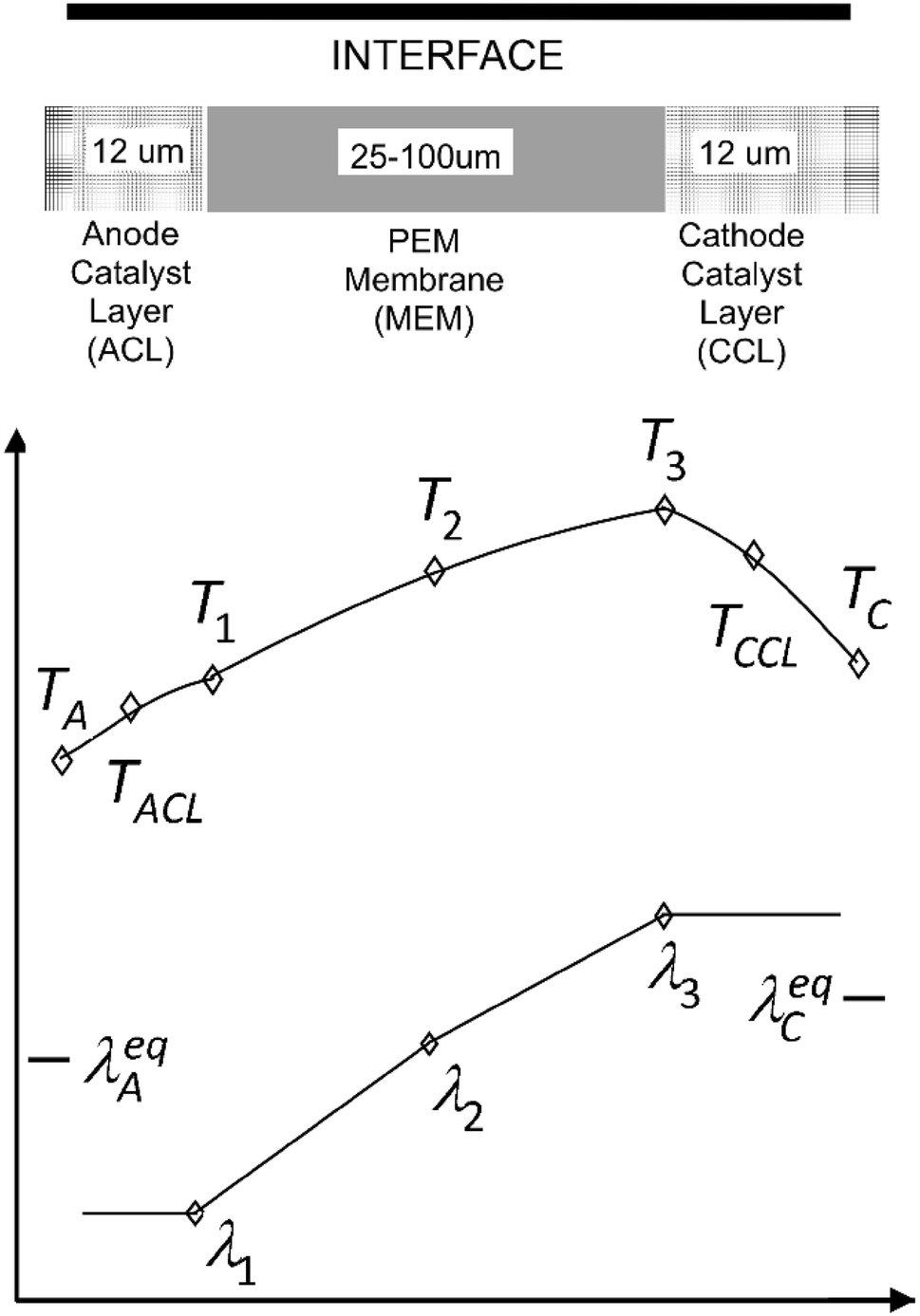
Figure ⁴ shows a profile schematic to explain the water and heat transport equations. An approximate water content profile λ(z) is assumed to be a second-order polynomial determined by three unknown values (λ1λ2λ3) occurring at the ACL–membrane interface (anode side), midpoint, and CCL–membrane interface (cathode side) of the membrane. The equilibrium water uptake of the anode, λAeq , and cathode, λCeq , are found using the water activity and temperature of the anode and cathode gases. The water contents of the ionomer in the ACL, λACL and CCL, λCCL , are assumed uniform throughout the respective catalyst layers, with the values of λ1 and λ3 .

Temperature and water content profile schematic of proposed interface model

The water transport model employs convective boundary conditions of water absorption and desorption. The MEA can gain or lose water content. The water content profile utilizes three equations: two values of its slope, at points 1 and 3, in addition to the integrated water content W , at pseudo-steady-state conditions. The pseudo-steady-state assumption involves ignoring water-content distribution variations within the ionomer of the MEA, to represent hydration level by an overall MEA water content.

The water contents are found by assembling three equations to solve for the three unknown water contents. The first equation relates the MEA water content W to the three water content values. The MEA water content W (mol m ⁻² ) is represented as a lumped parameter value for each cell of the interface. During steady-state operation, the value of W must be such that the water gain rate ∂W/∂t=0 . When W is less than the steady-state value, the water gain rate is positive; the converse occurs, as well. The overall water content of the ionomer phase, integrated through the thickness of the MEA can be presented as Eq. ( ⁹ ), which simplifies to Eq. ( ¹⁰ ):

W=∫z=-tACLz=tMEM+tCCLε(z)λ(z)dz=cfεACL,IotACLλ1+cftMEM6λ1+4λ2+λ3+cfεCCL,IotCCLλ3,

cftMEM+6cfεACL,IotACLλ1+4cftMEMλ2+cftMEM+6cfεCCL,IotCCLλ3=6W.

The second equation examines the slope in the water content profile at z = 0, the ACL–membrane interface. There is water flux to/from the ionomer by absorption or desorption from the anode gas stream, according to the absorption/desorption kinetics previously given. The water flux within the membrane should be identical, being driven by the combination of electroosmotic drag and back diffusion. The absorption flux (positive) or desorption flux (negative) is presented as Eq. ( ¹¹ ) and the water flux within the ionomer phase at z = 0 is written as Eq. ( ¹² ) using a three-point estimate of the slope at z = 0:

λAeq>λ1:JW,A=ka(fv,TACL)cf(λAeq-λ1)λAeq<λ1:JW,A=kd(fv,TACL)cf(λAeq-λ1),

\lambda_{1} :} & {J_{{{\text{W}},{\text{A}}}} = k_{\text{a}} (f_{\text{v}} ,T_{\text{ACL}} )c_{\text{f}} (\lambda_{\text{A}}^{\text{eq}} - \lambda_{1} )} \\ {\lambda_{\text{A}}^{\text{eq}} < \lambda_{1} :} & {J_{{{\text{W}},{\text{A}}}} = k_{\text{d}} (f_{\text{v}} ,T_{\text{ACL}} )c_{\text{f}} (\lambda_{\text{A}}^{\text{eq}} - \lambda_{1} ),} \\ \end{array} $$\end{document}]]>

JW,A=nd,1IF-cfDW,1dλdzz=0=nd,1IF-cfDW,1tMEM-3λ1+4λ2-λ3.

The expression simplifies to Eq. ( ¹³ ). The transport properties (drag coefficient nd,1 , diffusion coefficient DW,1 , and mass-transfer coefficient ka|d ) are evaluated at the water content and temperature of the ACL–membrane interface (λ1,T1) :

-3cfDW,1tMEMλ1+4cfDW,1tMEMλ2-cfDW,1tMEMλ3=nd,1IF-JW,A.

The third equation sets the slope in the water content profile at z=tMEM , the CCL–membrane interface. There is a water flux within the membrane driven by electroosmotic drag and back diffusion. Product water is produced in the ionomer phase of the CCL by the ORR. To the right of the CCL–membrane interface, there is desorption or absorption flux into or from the cathode gas stream. The desorption flux (positive) or absorption flux (negative) is presented as Eq. ( ¹⁴ ) where the water volume fraction term uses λ3 as the water content. The water flux within the ionomer phase at z=tMEM is written as Eq. ( ¹⁵ ) using a three-point estimate of the slope at z=tMEM :

λ3>λCeq:JW,C=kd(fv,TCCL)cf(λ3-λCeq)λ3<λCeq:JW,C=ka(fv,TCCL)cf(λ3-λCeq),

\lambda_{\text{C}}^{\text{eq}} :} & {J_{{{\text{W}},{\text{C}}}} = k_{\text{d}} (f_{\text{v}} ,T_{\text{CCL}} )c_{\text{f}} (\lambda_{3} - \lambda_{\text{C}}^{\text{eq}} )} \\ {\lambda_{3} < \lambda_{\text{C}}^{\text{eq}} :} & {J_{{{\text{W}},{\text{C}}}} = k_{\text{a}} (f_{\text{v}} ,T_{\text{CCL}} )c_{\text{f}} (\lambda_{3} - \lambda_{\text{C}}^{\text{eq}} ),} \\ \end{array} $$\end{document}]]>

JW,C=nd,3IF-cfDW,3dλdzz=tMEM=nd,3IF-cfDW,3tMEM3λ3-4λ2+λ1.

Water production by the ORR also occurs here. If interfacial resistance to water transport is incorporated into modeling efforts, a decision needs to be made as to where water creation occurs: in the CCL gaseous phase, ionomer phase, or directly as liquid. The extensive investigations of Wu et al. [ ²⁴ , ²⁵ ] have explained that water creation takes place in the ionomer phase.

The flux into the cathode, by electroosmotic drag and diffusion, is added to the product water creation, and set equal to desorption/absorption flux exiting the cathode into the cathode gas stream. Equating the water fluxes JW,C yields Eq. ( ¹⁶ ), where k3 is evaluated as an absorption or desorption coefficient according to the relative values of λCeq and λ3 . This expression simplifies to Eq. ( ¹⁷ ) where, again, the coefficients of diffusion ( DW,3 ) and electroosmotic drag ( nd,3 ) are evaluated at the water content and temperature of the CCL–membrane interface (λ3,T3) :

nd,3IF-cfDW,3dλdzz=tMEM⏟flux into CCL by EO drag / diffusion→+I2F⏟production in the CCL→=JW,C⏟desorption flux entering cathode gas stream→,

cfDW,3tMEMλ1-4cfDW,3tMEMλ2+3cfDW,3tMEMλ3=0.5+nd,3IF-JW,C.

Together, there is a system of three equations and three unknowns to solve for the water contents in Eq. ( ¹⁸ ). The solution updates (λ1λ2λ3) . The current density ( I ) is updated in a subsequent step. After the water content profile is calculated, the fluxes of water into the anode, JW,A , and out of cathode, JW,C , (mol m ⁻² s ⁻¹ ) can be updated from the water content profile of the MEA as Eq. ( ¹⁹ ):

3cfDW,1tMEM-4cfDW,1tMEMcfDW,1tMEM6cfεACL,IotACL+cftMEM4cftMEM6cfεCCL,IotCCL+cftMEMcfDW,3tMEM-4cfDW,3tMEM3cfDW,3tMEMλ1λ2λ3=JW,A-nd,1IF6W0.5+nd,3IF-JW,C,

JW,A=cfk1λAeq-λ1JW,C=cfk3λ3-λCeq.

The water gain rate within the MEA, ∂W/∂t (mol m ⁻² s ⁻¹ ), is found by applying conservation of mass principles to the water in the ionomer phase. In Eq. ( ²⁰ ), the first term represents water production due to the ORR; which takes place in the ionomer phase. The next term represents water flux into the anode and the final term water flux out of the cathode:

∂W∂t=I2F+JW,A-JW,C.

Gas-phase transport in catalyst layers

Gas transport losses within the anode and cathode catalyst layers are considered in this section. Hydrogen and oxygen reactants are consumed through the thicknesses of anode and cathode porous catalyst layers (electrodes). Reaction rates will vary with depth through the catalyst layer; however, the distribution of reaction rates is predominantly shaped by conduction losses in the catalyst layer’s ionomer [ ²⁶ , ²⁷ ] and not by normally occurring variations in reactant gas concentration. The reactant mole fractions at the outer edge of the ACL and CCL, XH2,A , and XO2,C are adjusted to diffusion-corrected values XH2,AD and XO2,CD at the location of average reaction current density as shown in Eqs. ( ²¹ ) and ( ²² ). The normal current density is I (A m ⁻² ); tACLD and tCCLD (m) represent the effective gas diffusion lengths within each catalyst layer, and DH2,ACLeff , DO2,CCLeff are the effective catalyst layer diffusion coefficients:

XH2,AD=XH2,A-I2FtACLDDH2,ACLeffRTACLPA,

XO2,CD=XO2,C-I4FtCCLDDO2,CCLeffRTCCLPC.

The through-plane gas-phase transport of the reactants occurs due to diffusion; pressure-driven flow is not considered. The consumption of reactants causes a gradient in the reactant mole fractions between the outer edge of the ACL/CCL and the membrane–catalyst layer interfaces. A simplified approach is employed; it assumes that all the reactants to be consumed (by stoichiometric requirements) must diffuse over an effective length. Effective length is treated as a known here, but it is determined analytically by conduction effects in a later section. The calculation details of the effective catalyst layer diffusion coefficients were given in [ ¹³ ]. Both molecular diffusion and Knudsen diffusion mechanisms must be accounted for. Porosity and tortuosity effects can be accounted for to produce an effective oxygen or hydrogen diffusivity. A reduction in mole fraction, at the catalyst layer’s mean reaction depth, can be calculated given the reactant flux necessary for the given current density.

Kinetics in catalyst layers

Kinetic losses, or activation losses, within the anode and cathode catalyst layers are considered in this section. These are the voltage losses required to drive the chemical reactions at the rate (current density) required. Anode kinetics typically is not that important to a PEMFC model as the hydrogen oxidation reaction (HOR) is quite facile, with a large exchange current density. Cathode kinetics is very important to PEMFC modeling and the subject of a great deal more research. The oxygen reduction reaction (ORR) occurring at the cathode is a source of major voltage loss with currently available practical PEMFC catalyst configurations. The kinetic models and parameters associated with each reaction need to be detailed. These are gathered from focused research in each area. This information is then subsequently used to calculate the ohmic loss terms within the MEA and estimate current density.

Anode kinetics

Anode kinetics follows the general Butler–Volmer (BV) model. The ideal BV model pre-supposes an anode catalyst layer (ACL) without ohmic resistance or gas diffusion losses [ ⁸ , ²⁸ ] in Eq. ( ²³ ), where I (A m ⁻² ) refers to the cell current and I0,A refers to the superficial exchange current density for the HOR occurring at the anode electrode (explained below). Here, the term ηA refers to the kinetic or activation overpotential at the anode (V): the voltage loss. The terms υa and υc are the anodic and cathodic charge transfer coefficients, respectively. These are fundamental constants describing the reaction, which are not supposed to change with operating conditions such as temperature, humidity, etc. [ ²⁹ , ³⁰ ]. They are not used here as adjustable parameters in a given problem. The superficial exchange current density I0,A is the dominant parameter in the BV equation to be influenced/optimized, influencing the voltage loss. Exchange current density depends on gas temperature, pressure, and reactant concentration (mole fraction). It also depends on electrode morphology, the catalyst type, and the aging/degradation of the catalyst layer. It is known to be an exponentially increasing function of temperature:

I=I0,AexpυaFRTACLηA-exp-υcFRTACLηA.

The HOR reaction is facile; the exchange current density can reach ~ 20 times or more the size of the maximum operating current density at typical operating conditions. The bracketed term must necessarily be small as well and so the arguments to the exponential terms are typically less than 0.15. With this limitation, the linearized BV equation in Eq. ( ²⁴ ) can represent the losses of the HOR [ ⁸ , ²⁸ ]:

ηA=RTACLυa+υcFII0,A.

Several sources indicate that the reaction is symmetric, i.e., υa=υc [ ²⁸ , ³⁰ , ³¹ – ³² ]. Sources indicate that υa=υc=0.5 , and thus, υa+υc=1 [ ⁸ , ²⁸ , ³⁰ ]. Other sources indicate that υa+υc=1 , and thus, υa+υc=2 [ ³¹ , ³² ]. Focused experiments [ ²⁹ ] claimed that both values of the charge transfer coefficients could fit the experimental data. As of 2015, Durst et al. showed that υa+υc=1 could fit measurements performed over a range of temperatures [ ³⁰ ].

The superficial exchange current density term, I0,A (A m ⁻² ), is a product of several factors in Eq. ( ²⁵ ); the form attempts to separate out and identify the different influences of temperature, gas concentration, catalyst layer morphology, and platinum loading. The exchange current density is proportional to the mole fraction of hydrogen XH2,AD present, at the mean reaction depth, in the anode catalyst layer. The term i0,ACL ( A cmPt-2 ) refers to the specific exchange current density of the HOR on platinum catalyst, expressed with the basis of the active area of platinum catalyst. It was reported [ ³⁰ ] to be between 0.24 and 0.26 ( A cmPt-2 ) at a temperature of 80 °C, and a temperature dependence was investigated. LACL,Pt (mg _Pt cm ⁻² ) is the anode platinum catalyst loading, known from the catalyst layer composition:

I0,A=1002XH2,ADi0,ACLLACL,PtAACL,Pt10.

The catalyst-specific exchange current density for the HOR on the carbon-supported platinum catalyst, i0,ACL ( A cmPt-2 ), has dependencies of temperature and hydrogen partial pressure in Eq. ( ²⁶ ). The term i0,ACL∗ represents the value at reference hydrogen partial pressure of 101 kPa and 80 °C (353 K) of 0.26 A cmPt-2 [ ²⁹ , ³⁰ ]. The activation energy of the HOR, EArev (kJ mol ⁻¹ ), was found to be 16 kJ mol ⁻¹ . The dependence of anode losses on hydrogen concentration is modeled through the diffusion-corrected hydrogen mole fraction XH2,AD present at the mean reaction depth in the ACL. Mass transport or diffusional losses result when H ₂ molecules cannot reach the CCL reaction sites to support the desired reaction rate. As XH2,AD diminishes, superficial exchange current density I0,A decreases and the anode overpotential ηA grows:

i0,ACL=i0,ACL∗PAXH2,AD101,300exp-EArevRTCCL1-TACL353.

The term AACL,Pt ( mPt2/gPt ) is the anode catalyst layer’s electrochemically available catalyst area, (ESA or ECSA), expressed per gram of catalyst, indicating morphology effects. This term measures the effectiveness of the catalyst layer microstructure and design in employing the catalyst to create maximum effective active area where the reaction can take place. It represents the surface area of the Pt catalyst that is simultaneously in contact with the reactant gas, the electronic conducting phase, and the proton conducting phase of the catalyst layer. It has been found to be typically 46–60 mPt2/gPt [ ⁷ , ⁸ ] at fully humidified conditions. Experiments with typical catalyst layer structures showed that this area could drop by 50% as humidity decreases from 100% RH to 50% RH [ ⁷ , ³³ , ³⁴ – ³⁵ ].

Carbon black supports, such as the commercially available product Vulcan XC-72 (Cabot Corp), were seen with relatively large pore-size distributions (PSD). Carbon supports with larger PSD tend to have higher ionomer coverage [ ³⁴ ] of the catalyst sites, and less reliance on surface-adsorbed water for proton conduction within the CL. For such a carbon black support, the ECSA is treated here as decreasing linearly with local CL water content λ , and not humidity [ ⁷ ], from 0 to 100% RH in Eq. ( ²⁷ ). This introduces more non-linearity into the problem of determining the current density and water contents within the MEA:

AACL,Pt=AACL,Pt100%RH1-0.91-λACL/λα=1,T.

This section described the HOR kinetic losses and superficial exchange current density I0,A (A m ⁻² ), occurring at the anode electrode. The purely kinetic losses of the anode are typically small and have been routinely ignored in modeling efforts [ ³⁶ ]. Ohmic losses in the ACL have not yet been considered; these can become significant under sub-saturated conditions. Combined ohmic and kinetic losses are needed, and will be addressed subsequently.

Cathode kinetics

BV kinetics simplify to Tafel kinetics when modeling the ORR occurring at the CCL. With very low exchange current density, and without significant conduction or diffusional losses, Tafel kinetics follows Eq. ( ²⁸ ) [ ³⁷ ] where the term ηC (V) refers to the purely kinetic or activation overpotential of the ORR at the cathode. I (A m ⁻² ) refers to the cell current as before and Ix the crossover current density (which represents a small amount of hydrogen permeation “crossover” from the anode through the membrane into the cathode). The term I0,C refers to the superficial exchange current density for the ORR occurring at the cathode electrode. Exchange current density for the ORR taking place on platinum catalyst depends on gas temperature, pressure, reactant concentration (mole fraction), electrode morphology, and the catalyst type. It is known to be an exponentially increasing function of temperature. The term υc is the cathodic charge transfer coefficient, which was found experimentally to be unity for the ORR when ohmic losses were correctly accounted for [ ³⁷ ]. The Tafel slope indicated is 70 mV/decade at 80 °C (with υc=1 ):

ηC=RTCCLυcFlnI+IxI0,C=2.303RTCCLυcF⏟Tafel SlopelogI+IxI0,C.

Experimental works have shown considerable disagreement in measuring the Tafel slope. Some works have reported “double Tafel slopes” where the values consistent with υc=1 are reported at low-current densities together with a doubled Tafel slope ( υc=0.5 ) at greater current densities. Prior CFD models, utilizing the interface approach, have employed doubled, or nearly doubled, Tafel slopes [ ³⁸ , ³⁹ ] for use with low-humidity conditions. In the present model, the cathodic charge transfer coefficient υc=1 and does not change with current level, humidity, or other factors.

The superficial exchange current density for the ORR I0,C (A/m ² ), occurring at the cathode electrode, is a product of several factors in Eq. ( ²⁹ ); this form attempts to separate the different influences of temperature, gas concentration, catalyst layer morphology, and platinum loading. I0,C is proportional to the mole fraction of oxygen XO2,CD present, at the mean reaction depth, in the anode catalyst layer. The term i0,CCL ( A cmPt-2 ) refers to the catalyst-specific exchange current density of the ORR on platinum catalyst, expressed with the basis of the active area of platinum catalyst. The term LCCL,Pt ( mgPt/cm2 ) is the cathode platinum catalyst loading, known from the catalyst layer composition, and ACCL,Pt ( mPt2/gPt ) is the cathode catalyst layer’s electrochemically available surface area (ECSA), which is as previously discussed for the anode:

I0,C=1002i0,CCLLCCL,PtACCL,Pt10.

The catalyst-specific exchange current density for the ORR on the carbon-supported platinum catalyst, i0,CCL ( A cmPt-2 ), has dependencies of temperature and oxygen partial pressure in Eq. ( ³⁰ ) where i0,CCL∗ represents the value at reference oxygen partial pressure of 101.3 kPa and 80 °C (353 K). It was found to be 2.5 × 10 ⁻⁸ [ ³⁷ ] and later 1.5 × 10 ⁻⁸ A cmPt-2 [ ⁷ ]. The kinetic reaction order with respect to oxygen partial pressure was found to be 0.54, and ECrev , the activation energy of the ORR (at zero overpotential/reversible cell potential), was found to be 67 kJ mol ⁻¹ :

i0,CCL=i0,CCL∗PCXO2,CD101,3000.54exp-ECrevRTCCL1-TCCL353.

Ohmic losses within the MEA

This section details the effective ohmic resistances present within the MEA. These resistances are needed for the current estimation. Ohmic losses within the interface are calculated from the hydration-dependent conductivities.

In situ high-frequency resistance (HFR) measurement produces RΩ (Ω m ² ) that is the sum of the membrane protonic resistance and the electronic resistances present as in Eq. ( ³¹ ). The HFR measurement is commonly used for the model validation of water transport modeling efforts, because the HFR measurement contains a first component that has membrane water-content dependence and a second component that has been found to be constant for a given cell assembly. The total ohmic resistance within the interface, ROhm (Ω m ² ), is the sum of HFR resistance and effective catalyst layer resistances as Eq. ( ³² ):

RΩ=RMEMH++Rcnte-,

ROhm=RΩ+RACLH+,eff+RCCLH+,eff=Rcnte-+RMEMH++RACLH+,eff+RCCLH+,eff.

Effective electronic resistance

The Interface model MEA contains electronic conduction resistances Rcnte- (Ω m ² ). This term is treated as a humidity-independent, but assembly-pressure-dependent, term. It can represent ACL/CCL electronic conduction losses and contact resistances between the gas diffusion media (GDL) and ACL/CCL (catalyst layers) at the outer edges of the MEA.

When comparing the interface model directly to experimental data, additional bulk resistances must be included in the electronic resistance term. Electronic bulk conduction losses may occur outside of the interface (MEA) region; in the anode and cathode diffusion media and the conductive flow-field plates. Electronic contact resistances can also be found between the diffusion media and flow-field plates.

Membrane resistance

The membrane proton conduction resistance RMEMH+ (Ω m ² ) is calculated by an approximate integration of the three hydration-dependent conductivity values. Volumetric swelling in the membrane is treated as occurring purely in the thru-plane direction (in thickness); membrane thickness swells with water content at the center at the membrane as following equation:

RMEMH+=∫0tMEMS1σIodz=tMEM1+εdV,261σIo,1+4σIo,2+1σIo,3.

Effective anode resistance

The voltage drop occurring in the ACL is modeled by an analytical solution which accounts for both kinetic and ohmic losses simultaneously. Kulikovsky [ ²⁸ ] developed an analytical solution for anode overpotential, in the absence of gas-phase diffusional losses (assuming ideal reactant transport), which will be expanded somewhat to account for ACL swelling which was not originally considered.

The ACL overpotential first depends on the ACL electrode sheet resistance, RACLH+,sheet (Ω m ² ). The sheet resistance of the anode is the protonic conduction resistance through the electrode, assuming that all current travels through the entire thickness of the electrode. The sheet resistance calculation in Eq. ( ³⁴ ) assumes that the ACL swells in thickness with water uptake. The term tACL (m) represents the CCL dry thickness, εACL,Io (–) the dry volume fraction of ionomer in the CCL, εdV,1 (–) the fractional volume swelling with water uptake at the anode side of the MEA, σIo,1 (Ω ⁻¹ m ⁻¹ ) the ionic conductivity calculated from water content and temperature, and τACL,Io (–) the tortuosity of the ionomer within the ACL. The tortuosity of the ACL ionomer conduction network is calculated in the same manner as for the CCL:

RACLH+,sheet=tACLτACL,Io1+εdV,1σIo,1εACL,Io.

The anode catalyst layer thickness can be viewed as being split into a conduction and diffusion thickness. The effective conduction thickness, tACLC , and the effective gas diffusion thickness, tACLD , sum to the swollen anode catalyst layer (ACL) thickness in Eq. ( ³⁵ ). The HOR reaction occurs within a thin strip at the membrane side of the ACL, and so, the ACL diffusional thickness is essentially the entire catalyst layer thickness. This effective diffusion length is used in Sect. ^2.6 to ascertain the reduction in reactant mole fractions within the anode catalyst layer:

tACLC≃0tACLD=tACL1+εdV,1.

The anode loss ηA (V) and the operating current density I are related as Eq. ( ³⁶ ), where σACLeff is the catalyst layer effective conductivity. The quantity under the radical is made small (< 1) by the large superficial exchange current density of the HOR, I0,A , making the sinh function nearly linear in character with respect to current density I . To a first approximation, overpotential ηA can vary linearly with current. The term I0,A will drop with diffusional reductions within the ACL, and with reductions in the ACL ionomer-phase water content (due to electroosmotic drag). The ACL conductivity σACLeff will also decline with increasing current density for the same reason. Accounting for the thickness expansion of the ACL, this formula can incorporate the effective anode sheet resistance RACLH+,sheet of the ACL as Eq. ( ³⁷ ):

ηA=RTACLυFsinh-1ItACLS2RTACLυFI0,AσACLeff,

ηA=RTACLυFsinh-1IRACLH+,sheet2RTACLυFI0,A.

If a small argument approximation is applied to linearize the arcsinh function, the relation can be re-written to appear explicitly linear as Eq. ( ³⁸ ). The ACL voltage losses have been assessed, experimentally, as being not completely linear with current density in a hydrogen concentration cell [ ¹⁹ , ²⁹ , ³⁰ ]. This last linearization is not employed here. The effective catalyst layer conduction resistance RACLH+,eff (Ω m ² ) is calculated from Eq. ( ³⁹ ), where the combined kinetic and ohmic losses of the ACL in Eq. ( ³⁸ ) are linearized to an effective resistance:

ηA=IRTACL2υFI0,ARACLH+,sheet=IRACLH+,kineticRACLH+,sheet,

RACLH+,eff=ηAI.

Finally, the bounds of validity of this anode loss approximation are addressed. This anode loss relationship was formed using a small argument simplification, described as the low-current approximation. The anode loss estimate has Eq. ( ⁴⁰ ) as a restriction on its validity:

IRACLH+,sheet2RTACLυFI0,A<coth2I0,ARACLH+,sheetRTACLυF=RACLH+,kineticRACLH+,sheetIRACLH+,sheetRTACLυF<cothRACLH+,sheetRACLH+,kinetic.

With practical ACL compositions, the right-most ratio is significantly greater than 1, and so, the coth function produces a result of very nearly unity. This relationship is thus valid when the ratio of ACL kinetic resistance RACLH+,kinetic to ACL sheet resistance RACLH+,sheet is suitably small in relation to the current density. It was noted that the PEMFC anode consistently obeys this low-current approximation, termed as the linear mode [ ²⁸ ]. Should ACL catalyst loading be greatly reduced, the validity of this relation needs to be re-assessed in terms of the reduced superficial exchange current density I0,A to be expected [ ⁴⁰ ].

Effective cathode resistance

The effective cathode catalyst layer resistance is derived from an analytical solution that was presented by Wang and Feng [ ²⁶ , ²⁷ ], as well as Neyerlin et al. [ ¹⁹ , ³⁷ ].

The analytical solution was developed incorporating several simplifying assumptions within the catalyst layers. The spatial distribution of all material phases (volume fractions) within the CL is assumed constant, as is the ionomer water content within the CCL, where there is constant ionic conductivity. Another key assumption of this analytical solution is that the solid phase, or electronic phase, is thought to have constant phase potential through the thickness of the electrode; electrical conduction losses are assumed insignificant. Electrical contact resistances were incorporated at the outer edge of the catalyst layers. The CCL is assumed to be effectively isothermal [ ²⁶ ]. Under these conditions, variations in reaction rate within a porous electrode are dependent upon conduction losses and the Tafel slope of the reaction.

Reactant gaseous concentration levels are assumed to be constant within the variable depth of the catalyst layer, which is also referred to as the absence of O2 diffusion resistances. Wang and Feng estimated that, in most ranges of fuel cell operation, diffusional losses within the CCL would be insignificant [ ²⁶ ]. Detailed numerical analysis of the reaction rate distribution throughout the thickness of a PEMFC catalyst layer has also been performed by modeling. Wu et al. carried out the full analysis numerically, and found that reaction rates located to minimize conduction losses, without noticeable impact from gas concentration losses [ ⁴¹ ]. This was said to be due to the form of the Butler–Vollmer equation, where the variations in the exponential term (for overpotential) had much more impact on reaction rates than the variations in the linear term (where exchange current density carries a linear dependence on the gaseous reactant concentration term). This work utilizes this analytical solution, but with the small diffusional correction of Sect. ^2.6 applied.

The electrode sheet resistance RCCLH+,sheet (Ω m ² ) in Eq. ( ⁴¹ ) expresses the effective protonic conduction resistance through the electrode, assuming that all current travels through the entire thickness of the electrode, where the electrode swells in thickness with water uptake as the membrane does. The term tCCL (m) represents the CCL dry thickness, εCCL,Io (–) the dry volume fraction of ionomer in the CCL, εdV,3 (–) the fractional volume swelling with water uptake at the cathode side of the MEA, σIo,3 (Ω ⁻¹ m ⁻¹ ) the ionic conductivity calculated from water content and temperature, and τCCL,Io (–) the tortuosity of the ionomer within the CCL. Details about the calculation of tortuosity are given in [ ¹³ ]:

RCCLH+,sheet=tCCLτCCL,Io1+εdV,3σIo,3εCCL,Io.

A dimensionless performance parameter θCCL in Eq. ( ⁴² ) is the ratio of proton conduction resistance to kinetic resistance within the CCL [ ¹⁹ ]. The numerator includes the sheet resistance and current density. The denominator is the Tafel slope of the ORR expressed as b in V/decade. It has been found as 70 mV/decade at 80 °C [ ³⁷ ]:

θCCL=IRCCLH+,sheet2.303RTCCL1F=RCCLH+,sheetb/I=RCCLH+RCCLη.

The effective catalyst layer conduction resistance RCCLH+,eff (Ω m ² ) is then calculated from the sheet resistance RCCLH+,sheet and the resistance correction factor as χCCL(θCCL) as Eq. ( ⁴³ ) [ ¹⁹ ]. The correction factor χCCL(θCCL) is fit with an approximate function in Eq. ( ⁴⁴ ) valid between 0 and 30. Values below and above that range were limited to 1 and 5.908, respectively:

RCCLH+,eff=13RCCLH+,sheetχCCL(θCCL),

χCCL(θCCL)=1.008+0.2371θCCL-0.00236θCCL2.

The thickness of cathode catalyst layer can then be viewed as being split into a conduction and diffusion thickness. The effective conduction length, tCCLC , and the effective gas diffusion length, tCCLD , are defined by Eqs. ( ⁴⁵ ) and ( ⁴⁶ ). This effective diffusion length is used in Sect. ^2.6 to ascertain the reduction in reactant mole fractions within the cathode catalyst layer:

tCCLC=tCCL1+εdV,313χCCL(θCCL)

tCCLD=tCCL1+εdV,31-13χCCL(θCCL).

Polarization curve and current estimation

This section describes the voltage–current relationships in the interface model. Established voltage and current relationships are used to produce an updated estimate of current density with the Newton–Raphson technique.

The thermodynamically determined open circuit, ideal, or reversible voltage can be calculated from the established thermodynamic relationships. The relationship used in this work was given by Liu et al. [ ⁷ ]. The reversible cell voltage VOC is Eq. ( ⁴⁷ ). The reversible cell voltage can be seen to be a function of cathode temperature ( TCCL ), hydrogen partial pressure ( XH2,ADPA ), oxygen partial pressure ( XO2,CDPC ), and cathode humidity αC . The definition of the open-circuit voltage takes into account some reduction in the oxygen and hydrogen mole fractions due to mass-transfer (diffusional) losses within the catalyst layers:

VOC=1.229-0.000846TCCL-298+RTCCL2FlnXH2,ADPA101,300+RTCCL4FlnXO2,CDPC101,300-RTCCL2FlnαC.

The cell voltage in Eq. ( ⁴⁸ ) is the difference between cathode ( VC ) and anode ( VA ) potential levels. Cell current is the previously described current density. The cell voltage is the ideal/reversible voltage minus various voltage losses [ ¹⁹ ]. The ACL combined kinetic and ohmic losses have been incorporated into RACLH+,eff within the ohmic resistance term ROhm . The iR-free or kinetic voltage Vk in Eq. ( ⁴⁹ ) describes the cell voltage in the absence of ohmic losses. The kinetic voltage is formed analytically by subtracting cathode kinetic losses ηC from VOC :

Vcell=VC-VA=VOC-IROhm-ηC,

Vk=VOC-ηC≈Vcell+IROhm.

The voltage loss Vloss is defined as a simple re-arrangement to give Eq. ( ⁵⁰ ), which is the voltage–current relationship of the interface, where the current density I needed to satisfy this relationship is sought, but is not known. An implementation of the Newton–Raphson root-finding method to solve for the current density Inew was found sufficiently stable for use here. The procedure initializes I=Ix and then calculates an updated estimate of the operational current density Inew using Eq. ( ⁵¹ ):

Vloss=VOC-Vcell=IROhm+RTCCL1FlnI+IxI0,C,

Inew=I+Vloss-IROhm-RTCCL1FlnI+IxI0,CROhm+RTCCL1FI+Ix.

MEA thermal treatment

The interface takes as inputs the temperatures from the opposite sides of the MEA and outputs heat fluxes to the anode and cathode computational domains. Some earlier interface models created a thermal source term at the cathode GDL/MEA interface based upon the (estimated) overall efficiency of the device [ ⁴² ]. This present model divides the heat flux between anode and cathode, but does not go into high detail examining the spatial distribution of heat generation within catalyst layers. It is included, because several terms from the interface model were given temperature-dependent.

A 1-D temperature profile estimates the temperature rise in the MEA in Fig. ⁴ . Temperatures TA and TC are taken as Dirichlet boundary conditions from the 3D simulation as thermal contact resistance is thought to be minimal. A simultaneous solution of the seven temperature values (five unknowns) is developed to produce a steady-state temperature profile and heat fluxes into the anode and cathode flow domains.

This section applies a general heat transport equation to the MEA. Heat generation within the regions of the MEA has been detailed [ ⁴³ ]; it typically occurs predominantly within the CCL. The thermal conductivities and heat generation terms of each region of the MEA are collected. Convective effects within the MEA are ignored, following similar work [ ⁴⁴ ]. Heat transport in the thru-plane direction occurs by conduction, with the thermal conductivity being hydration-dependent. The regions of the MEA are thought to be isotropic and thermal contact resistances between the layers of the MEA are thought to be negligible [ ⁴⁵ ].

The governing equation of heat transport can be written as Eq. ( ⁵² ), where κieff refers to the thermal conductivity (W m ⁻¹ K ⁻¹ ), T the temperature (K), Q˙i the superficial heat source (W m ⁻² ), and ti (m) the layer thickness. The subscript i refers to the three regions of the MEA ( i = ACL, MEM, CCL). Details of thermal conductivities, κieff , of the MEA regions are given in [ ¹³ ]:

J→T,i=-κieff∇T;∇·-κieff∇T=Q˙iti.

Estimates of the superficial heat generation, Q˙i , within the regions of the MEA, are available [ ²⁴ , ⁴⁴ ]. Within the anode catalyst layer, heat generation occurs from irreversible heating sources. The combined kinetic and ohmic ACL losses will generate heat, in addition to half of the MEA electronic resistance. The anode superficial heat generation is expressed as Eq. ( ⁵³ ) where the ACL swells in thickness with water uptake:

Q˙ACL=I2RACLH+,eff+Rcnte-/2.

Within the membrane, there is only the irreversible heat source of ohmic losses (protonic conduction losses). The membrane superficial heat generation is expressed by the following equation:

Q˙MEM=I2RMEMH+.

The cathode catalyst layer has both reversible and irreversible heat sources in Eq. ( ⁵⁵ ). Reversible heat generation in the CCL stems from the entropy change of the overall reaction, and irreversible heat generation from the cathode activation (kinetic) and ohmic losses. The entropy change of the reaction, dS (= 44 J mol ⁻¹ K ⁻¹ ), assumes that produced water exits the MEA in vapor form [ ⁸ , ²⁴ , ³² ], and is approximately constant at temperatures below 100 °C. The term ηC represents the purely kinetic losses in the cathode as described earlier. The right-most term represents ohmic heat generation, utilizing the effective cathode resistance and half of the MEA electronic conduction resistance:

Q˙CCL=ITCCLdS4F+IηC+I2RCCLH+,eff+Rcnte-/2.

The temperature profile within the MEA is now to be determined. Referring to Fig. ⁴ , there are seven temperature values in the approximate profile, and thermal contact resistances are negligible [ ⁴⁵ ]. The regional heat sources are approximately uniform (within each region). The temperature profile can be expressed as the solution to a system of five heat transfer equations with the five unknown temperatures.

The conservation of energy equation, Eq. ( ⁵² ), is applied to the anode catalyst layer in Eq. ( ⁵⁶ ), the membrane in Eq. ( ⁵⁷ ), and the cathode catalyst layer in Eq. ( ⁵⁸ ):

4κACLefffv,TtACL1+εdV,12TA-2TACL+T1=-Q˙ACLtACL1+εdV,1,

4κMEM,2efffv,TtMEM1+εdV,22T1-2T2+T3=-Q˙MEMtMEM1+εdV,2,

4κCCLefffv,TtCCL1+εdV,32T3-2TCCL+TC=-Q˙CCLtCCL1+εdV,3.

A continuity of heat flux requirement can be applied at the ACL–membrane interface in Eq. ( ⁵⁹ ) and the membrane–CCL interface in Eq. ( ⁶⁰ ):

-κACLeff∇TACL=-κMEM,1eff∇TMEMκACLefffv,TtACL1+εdV,1TA-4TACL+3T1=κMEM,1efffv,TtMEM1+εdV,2-3T1+4T2-T3,

-κMEM,3eff∇TMEM=-κCCLeff∇TCCLκMEM,3efffv,TtMEM1+εdV,2T1-4T2+3T3=κCCLefffv,TtACL1+εdV,3-3T3+4TCCL-TC.

After re-arrangement and simplification, the temperature profile can be expressed as Eq. ( ⁶¹ ). The term Θ-CL is the ratio of thermal (conduction) resistance of the catalyst layers to that of the ionomer membrane as Eq. ( ⁶² ). The boundary heat fluxes into the anode JT,A and cathode JT,C domains can be solved for in Eq. ( ⁶³ ), again using three-point approximations to the first derivative of the temperature profile:

2-10004-31+ΘACL4ΘACL-ΘACL00-12-100-ΘCCL4ΘCCL-31+ΘCCL4000-12TACLT1T2T3TCCL=TA+Q˙ACLtACL1+εdV,14κACLefffv,TTAQ˙MEMtMEM1+εdV,24κMEM,2efffv,TTCTC+Q˙CCLtCCL1+εdV,34κCCLefffv,T,

ΘACL=κMEM,1efftACLκACLefftMEMΘCCL=κMEM,3efftCCLκCCLefftMEM,

JT,A=-κACLefffv,TtACL1+εdV,13TA-4TACL+T1JT,C=-κCCLefffv,TtCCL1+εdV,33TC-4TCCL+T3.

Boundary conditions

When the iterative scheme of the previous sections converges on a MEA current density estimate, temperature profile, and water-content profile, the interface model produces its outputs to the 3-D computational domains. Boundary conditions on the anode and cathode side of the MEA represent current density, heat flux, reactant consumption, and water flux in Eq. ( ⁶⁴ ). Water content is also updated:

Je,A=IJe,C=-IJT,A=-κACLefffv,TtACL1+εdV,13TA-4TACL+T1JT,C=-κCCLefffv,TtCCL1+εdV,33TC-4TCCL+T3NH2,A=-I2FMH2NO2,C=-I4FMO2NH2O,A=-JW,AMH2ONH2O,C=JW,CMH2ONm,A=NH2,A+NH2O,ANm,C=NO2,C+NH2O,C.

Iterative operation

This section describes the iterative operation of the interface model. As described, this algorithm can be run within a general-purpose computing package such as MATLAB. The main variables of the iterative routine are given in Table ⁴ . In the inner loop, the water content W and water fluxes JW,- are held constant, when the remaining variables are solved for.

Table 4

Principal interface variables for iterative solution

Symbol	Description
{λ1λ2λ3}	Water content profile
{JW,A, JW,C}	Water fluxes
{W}	Water content of the ionomer phase of the MEA
{I}	Current density
{TACL, T1-T3, TCCL}	Temperature profile
{JT,A, JT,C}	Thermal fluxes

First, the water content profile λ1λ2λ3 is determined. Then, volume fractions within the ionomer are calculated. Water transport parameters are then determined for the ionomer phase. The water transport equations are then solved with the most recent estimates of current density and the other solution variables. Second, the MEA ohmic resistances are re-assessed. Effective membrane, anode, and cathode resistances are updated from the water content profile. Third, gas-phase diffusional adjustments, representing mass-transfer resistances within the catalyst layers, are found. The diffusion-corrected oxygen and hydrogen mole fractions are then calculated. Fourth, the current density estimate I is updated. Finally, the MEA temperature profile is updated.

The outer loop operates to adjust overall hydration and boundary water flux values, in addition to the remaining boundary conditions described in the previous section. These calculations run only after a converged estimate of current density I is achieved within the inner loop. Water fluxes JW,A and JW,C are updated, but with relaxation factor (~ 0.5) to ensure stability and convergence. Water content W is updated with a pseudo time step (~ 0.25–0.5 s). The water gain rate ∂W/∂t will approach zero as W nears its equilibrium value.

The convergence of the algorithm was assessed with two criteria: current density and water gain rate. Verification cases produced convergence of the MEA current density { I } to within ~ 1% in a few (~ 5) iterations of the inner loop. The outer loop iterates to adjust overall hydration. Meaningful steady state, or equilibrium, is reached only when ∂W/∂t goes below a tolerance such as 0.00005 mol m ⁻² s ⁻¹ . The number of iterations required varies principally from starting value of W chosen. Typically, 10–30 iterations are observed.

Model validation

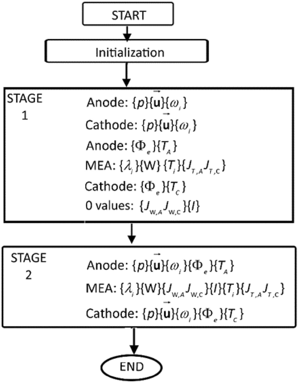
The Non-equilibrium Interface Model of membrane-electrode assembly (MEA) behavior is validated through the use of a previously published experimental data set from Neyerlin et al. [ ¹⁹ ]. The interface model is intended to simulate the localized behavior of a larger device, but here is validated against a small-area PEMFC with spatially uniform flow conditions. The experiment requires well-defined MEA compositions to be meaningful. Solutions here consider only effects in the thru-plane direction and ignore variations of input parameters (properties) in the planar directions, treating those conditions as locally uniform. Figure ⁵ shows a flowchart of the solution scheme.

With uniform conditions within the anode and cathode gas streams, model predictions are compared against the measurements of cell ohmic resistance and the several voltage components. The voltage components are generally divided and described according to their respective loss mechanisms. Kinetic losses of the cathode’s ORR reaction are presented as the first loss mechanism. Some discrepancies exist in the treatment of these losses. Ohmic losses of the membrane are the second loss mechanism. Cell ohmic resistance measurements reflect changes in hydration levels of the membrane. Ohmic losses associated with the ACL and CCL are also assessed. The measured cell voltage is shown with and without correction for high-frequency resistance (HFR).

The differential PEMFC was built with small planar dimension (i.e., 0.5 cm ² ) and operated with gas flows of very high stoichiometry (10–100). The intention is to create aforementioned conditions as uniform as possible within the anode and cathode. The collection of experiments was performed to examine voltage losses within the cathode catalyst layer under operating conditions where full 100% catalyst utilization does not occur. The sources of voltage loss could be concurrently assessed (with catalyst layers of well-defined composition). For the purposes (here) of developing a useful interface model, a means of estimating ACL and CCL losses under all relevant operating conditions is needed. This validation step provides a means of checking the model’s estimates against relevant experimental data.

The experiment explicitly made the assumption that diffusional losses within the differential PEMFC could be neglected, an assumption which sets the gas pressures, temperatures, and mole fractions from the inlet(s) of the anode and cathode as the same as those adjacent to the MEA. Diffusional losses within the catalyst layers are similarly not considered by the experiment. The task of estimating ACL/CCL losses is then contemplated as estimating the effective protonic conduction resistance(s) within the ACL and CCL. Temperature rise was not considered. Temperature rise and diffusional losses within the MEA are estimated, however, by the interface model.

Experimental conditions

Operating conditions are shown in Table ⁵ . Humidified hydrogen and oxygen were used as reactant gases. The gases were 100% humidified and 60% humidified at T = 80 °C. Hydrogen and oxygen partial pressures were reported as 101 kPa, and hydrogen and oxygen partial pressures were identical. The saturation pressure of water vapor is 47.79 kPa at 80 °C, and therefore, the total pressures are 149/130 kPa for the cases of 100%/60% RH. Constant gas flow rates of 1050 sccm for hydrogen and 600 sccm for oxygen feeds were used, guaranteeing minimum stoichiometric ratios of 20 (anode) and 23 (cathode) at the largest current density of 1.5 A/cm ² . The uniformly high stoichiometric ratio of the gas flows should create spatially uniform water and current distribution within the plane of the MEA, creating the sought after differential cell flow condition. The pressure drop from inlet to outlet was reported as only 3 kPa or less; it is not considered further.

Table 5

Operating conditions and parameters from the water transport validation experiment

Parameter	Symbol	Value
Operating cell voltage	VcellOP	0.87–0.76 V
Average current density	IcellOP	0.030–1.0, 1.25, 1.5 A cm⁻²
MEA area (length × width)	AMEA	5 cm²

Anode			Cathode
Parameter	Symbol	Value	Parameter	Symbol	Value
Operating pressure	PAOP	Case 1: 149.09 kPa Case 2: 129.95 kPa	Operating pressure	PCOP	Case 1: 149.09 kPa Case 2: 129.95 kPa
Stoichiometric flow ratio	ζAOP	20.0 (min)	Stoichiometric flow ratio	ζCOP	23.0 (min)
Relative humidity	RHAOP	Case 1: 100% Case 2: 60%	Relative humidity	RHCOP	Case 1: 100% Case 2: 60%
Inlet temperature	TAOP	353.15 K	Inlet temperature	TCOP	353.15 K
Cell temperature	TAOP	353.15 K	Cell temperature	TCOP	353.15 K

The mol fractions of hydrogen/oxygen, water vapor, and inert nitrogen are calculated from their respective partial pressures. The relevant gas pressures and mole fractions settings are shown below in Table ⁶ .

Table 6

Gas input compositions of anode and cathode from the water transport validation experiment

Case 1: 80 °C temperature 101 kPa reactant partial pressures 100% RH	Anode VA = 0	pH2 = 101 kPa	pH2O = 47.79 kPa	pN2 = 0 kPa	pA = 149.09 kPa
	Anode VA = 0	xH2,A = 0.679	xH2O,A = 0.320	xN2,A = 0.0
	Cathode VC = 0.66–0.90	pO2 = 101 kPa	pH2O = 47.79 kPa	pN2 = 0 kPa	pC = 149.09 kPa
	Cathode VC = 0.66–0.90	xO2,C = 0.679	xH2O,C = 0.320	xN2,C = 0.0
Case 2: 80 °C temperature 101 kPa reactant partial pressures 60% RH	Anode VA = 0	pH2 = 101 kPa	pH2O = 28.65 kPa	pN2 = 0 kPa	pA = 129.95 kPa
	Anode VA = 0	xH2,A = 0.779	xH2O,A = 0.220	xN2,A = 0.0
	Cathode VC = 0.55–0.89	pO2 = 101 kPa	pH2O = 28.65 kPa	pN2 = 0 kPa	pC = 129.95 kPa
	Cathode VC = 0.55–0.89	xO2,C = 0.779	xH2O,C = 0.220	xN2,C = 0.0

The differential PEMFC, with active area of 5 cm ² , was formed by two graphite interdigitated flow fields compressing the respective anode and cathode diffusion media (DM) and MEA between them. A Teflon gasket was utilized to seal the perimeter. The diffusion media were carbon fiber paper substrates (Toray, Inc.) subsequently hydrophobized with polytetrafluoroethylene (PTFE) and given an un-described surface treatment. Their thickness and composition is not further described, because that work assumes the absence of oxygen diffusion losses in these DM. Table ⁷ shows the MEA composition. The membrane has 1100 equivalent weight (EW) Nafion ionomer with a nominal thickness of 25 μm which is quoted at 50% RH. For modeling purposes, a dry thickness of 22 μm is used as that corresponds to a swollen membrane thickness of 25 μm at 50% RH. A crossover current density of 1 mA/cm ² was assumed here.

Table 7

MEA compositions compiled from the experiment

Membrane	Ionomer equivalent weight	EW	1100	g/mol SO₃⁻
	Thickness (dry)	tMEM	22 × 10⁻⁶	m
	Crossover current density	Ix	10	A/m²
Anode catalyst layer	Platinum loading	LACL,Pt	0.35	mg_Pt/cm²
	Pt/C mass ratio	PtcACL	50	%
	Ionomer-to-carbon ratio	ICACL	1.4	–
	Thickness (dry)	tACL	12 × 10⁻⁶	m
	Available catalyst area	AACL,Pt100%RH	50	mPt2/gPt
	Specific exchange current density	i0,ACL∗	0.24	A/cmPt2
Cathode catalyst layer	Platinum loading	LCCL,Pt	0.5	mg_Pt/cm²
	Pt/C mass ratio	PtcCCL	50	%
	Ionomer-to-carbon ratio	ICCCL	1.4	–
	Thickness (dry)	tCCL	18 × 10⁻⁶	m
	Available catalyst area	ACCL,Pt100%RH	50	mPt2/gPt
	Specific exchange current density	i0,CCL∗	2 × 10⁻⁸	A/cmPt2
Electronic	Cell electronic resistance	Rcnte-	0.034	Ω cm²

The anode catalyst layer (ACL) has platinum loading of 0.35 mg _Pt /cm ² and a thickness of 12 μm. It was made from carbon-supported PT catalyst with 50% Pt/C mass ratio. The ionomer-to-carbon ratio was 1.4, which yielded nearly the given ionomer volume fraction of 0.2. The cathode catalyst layer (CCL) has platinum loading of 0.50 mg _Pt /cm ² and a thickness of 18 μm.

An estimate of the purely electronic resistances within the differential PEMFC was created experimentally. A dummy cell was created from the differential PEMFC when the MEA was removed and the device reassembled. Electrical resistance measurements of the dummy cell were used to estimate the PEMFC electrical resistances. The electronic conduction losses are considered constant, independent of temperature and humidity effects. The supplied resistance value (0.030 Ω cm ² ) was adjusted upward, slightly, to (0.034 Ω cm ² ) compensate for the contact resistances between the GDL and MEA (missing from the dummy cell’s resistance measurement).

Polarization curves were measured at 11 points with current densities of 0.03, 0.045, 0.065, 0.1, 0.2, 0.3, 0.5, 0.75, 1.0, 1.25, and 1.5 A/cm ² . Measurements of HFR were performed after each point, as well. A separate test estimated the hydration-dependent voltage losses of the anode. Hydrogen-pump measurements, performed under identical pressure and humidity operating conditions, provided an estimate of the voltage loss associated with the combined kinetic and conduction losses within the anode of the PEMFC. The voltage losses appeared as almost constant resistances, with the low-humidity case presenting, as expected, a greater effective resistance.

Comparison of results

Interface model results are compared against the published experimental data. The experimental work reported, for the conditions given, the cell voltage VC-VA , current density I , exchange current density Ix , high-frequency resistance (HFR) RΩ , and electronic resistance Rcnte- measured from an empty “dummy cell”. Diffusional resistances anywhere in the cell, whether the GDL or the cathode catalyst layer, were neglected in the work.

The HFR-corrected voltage is the sum of the measured cell voltage and measured cell ohmic losses (from HFR) as in Eq. ( ⁶⁵ ). The kinetic voltage was found experimentally by adding the HFR-corrected voltage to ohmic corrections accounting for protonic conduction losses in the anode and cathode catalyst layers, in Eq. ( ⁶⁶ ), where RACLH+,eff and RCCLH+,eff are the effective anode and cathode catalyst layer resistances, respectively:

VHFR - corrected=Vcell+IRΩ,

Vk=Vcell+IROhm=Vcell+IRΩ+IRACLH+,eff+IRCCLH+,eff.

The anode effective resistance RACLH+,eff was estimated from separate hydrogen-pump experiments. To determine RCCLH+,eff , they assumed that the average membrane conductivity, measured by the high-frequency resistance measurement, could also be used to describe the average conductivity of the ionomer phase of the cathode catalyst layer. With knowledge of the thickness of each region ( tCCL and tMEM ), and the ionomer volume fraction of the CCL, εCCL,Io , the effective cathode catalyst layer resistance is Eq. ( ⁶⁷ ), where it was assumed in the previous work that the tortuosity of the ionomer conduction network in the CCL electrode is unity. The kinetic voltage becomes Eq. ( ⁶⁸ ):

RCCLH+,eff=13RΩ-Rcnte-χCCL(θCCL)εCCL,IotCCLtMEM,

Vk=Vcell+IRΩ+IRACLH+,eff+13RΩ-Rcnte-εCCL,IotCCLtMEM.

The interface model was used to create results at current density values comparable to the experiment. The water gain rate in the MEA, ∂W/∂t , is nearly zero (< 5 × 10 ⁻⁵ , or several orders of magnitude lower than the water content), indicating that the water content has reached equilibrium. For the 100% RH case, W decreases with current density from anode dryness. At 60% RH, the model predicts the opposite trend.

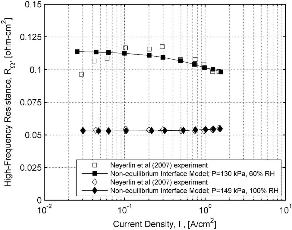
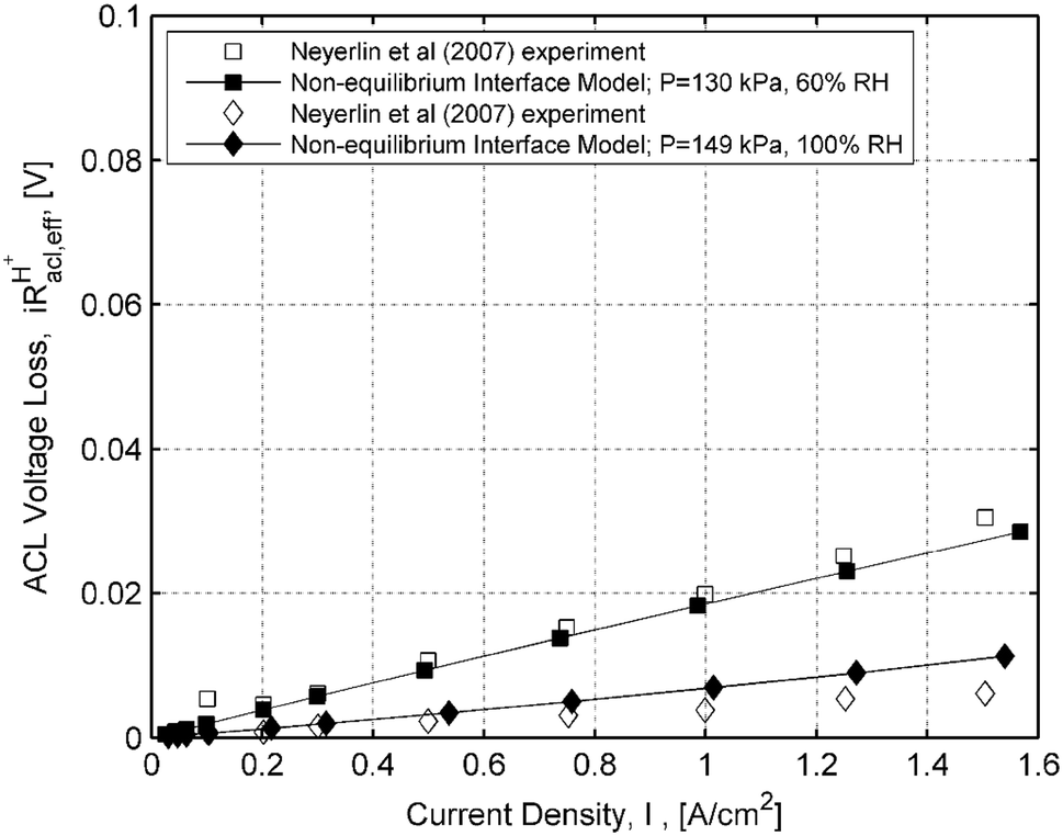
HFR measurements are compared against the interface model in Fig. ⁶ . Experimental results at 60% RH show greater variation with current density than those at 100% RH. Though resistance readings below 0.1 A/cm ² might be unreliable, HFR measurements at 60% RH show a drop with increasing current density. This drop is reproduced correctly by the model. It is the drop in resistance with decreasing current density, seen in the experiments, that is not reproduced by the model. It is not clear if this is due to experimental error or model deficiency. The HFR predictions at 100% RH now reflect the experimental data where resistance levels increase from 0.053 to 0.055 Ω cm ² at 1–1.5 A/cm ² .

Measured HFR and calculations of HFR from the interface model

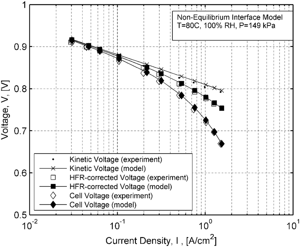
Voltage measurements are compared against the interface model at 100% RH in Fig. ⁷ . In the figure, the kinetic voltages predicted by this model utilize the active catalyst area given by the experiment. The gap between kinetic voltages and HFR-corrected voltages, predicted by this model, indicates a correct assessment of the summed ACL + CCL effective resistances. Thus, the non-equilibrium model accounts for the effective catalyst layer resistances correctly. The HFR predictions at 100% RH agreed well with the experimental values, and hence, the gap between cell voltage and the HFR-corrected voltage is also equal in both model and experiment. It follows that cell voltage levels show good agreement with measured values.

Measured and modeled voltages from the non-equilibrium interface at 100% RH

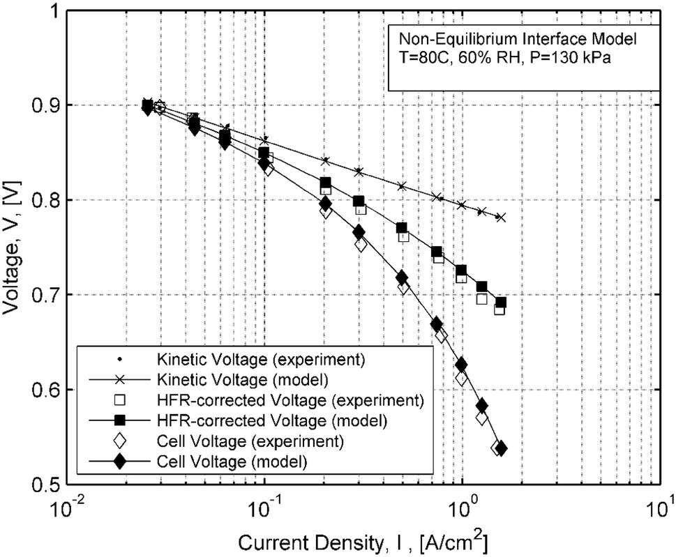
Voltage measurements are compared against the non-equilibrium interface model at 60% RH in Fig. ⁸ . The gap between kinetic voltages and HFR-corrected voltages, predicted by this model, indicates a slight underestimation of the summed ACL + CCL losses. The HFR predictions agreed well with the experimental values, and hence, the gap between cell voltage and HFR-corrected voltage is also equal between model and experiment. The resulting cell voltage levels from the model are slightly above experimental values due to the slight underestimation of the effective ACL resistance. The differences typically were under 6–10 mV, which is similar to the amount of scatter found in the testing of the underlying cathode kinetic loss relationships [ ³⁷ ].

Measured and modeled voltages from the interface model at 60% RH

Anode voltage loss, through a hydrogen-pump test, was also reported for both cases. Anode losses were reported as 30 mV at 1.5 A/cm ² , or = 0.02 Ω cm ² for the low-humidity case, and only reached 5 mV in the high-humidity case. Figure ⁹ shows anode voltage loss data against the model predictions. Anode losses of the low-humidity case are correctly assessed, while the very small anode losses of the high-humidity case were predicted as greater than the experimentally derived values. ACL conduction losses are frequently ignored entirely; this minor disagreement is not deemed critical.

Measured and modeled anode losses from the interface model

Publisher's Note

Springer Nature remains neutral with regard to jurisdictional claims in published maps and institutional affiliations.

Interface model of PEM fuel cell membrane steady-state behavior

Abstract

Introduction

Fig. 1

References

Wang et al. (2011) A review of polymer electrolyte membrane fuel cells: technology, applications, and needs on fundamental research 88(4) (pp. 981-1007) 10.1016/j.apenergy.2010.09.030
Guvelioglu and Stenger (2005) Computational fluid dynamics modeling of polymer electrolyte membrane fuel cells 147(1–2) (pp. 95-106) 10.1016/j.jpowsour.2005.01.011
Bednarek and Tsotridis (2017) Issues associated with modelling of proton exchange membrane fuel cell by computational fluid dynamics (pp. 550-563) 10.1016/j.jpowsour.2017.01.059
Carnes et al. (2013) Validation of a two-phase multidimensional polymer electrolyte membrane fuel cell computational model using current distribution measurements (pp. 126-137) 10.1016/j.jpowsour.2013.02.039
Dutta et al. (2001) Numerical prediction of mass-exchange between cathode and anode channels in a PEM fuel cell (pp. 2029-2042) 10.1016/S0017-9310(00)00257-X
Wang (2004) Fundamental models for fuel cell engineering 104(10) (pp. 4727-4766) 10.1021/cr020718s
Liu et al. (2009) Proton conduction and oxygen reduction kinetics in PEM fuel cell cathodes: effects of ionomer-to-carbon ratio and relative humidity 156(8) (pp. B970-B980) 10.1149/1.3143965
Jalani et al. (2005) TEOM: a novel technique for investigating sorption in proton-exchange membranes 254(1–2) (pp. 31-38) 10.1016/j.memsci.2004.12.020
Jalani and Datta (2005) The effect of equivalent weight, temperature, cationic forms, sorbates, and nanoinorganic additives on the sorption behavior of Nafion® 264(1–2) (pp. 167-175) 10.1016/j.memsci.2005.04.047
Zawodzinski et al. (1993) A comparative study of water uptake by and transport through ionomeric fuel cell membranes 140(7) (pp. 1981-1985) 10.1149/1.2220749
Walsby et al. (2002) Water in different poly(styrene sulfonic acid)-grafted fluoropolymers 86(1) (pp. 33-42) 10.1002/app.10832
Unknown ()
Kusoglu et al. (2011) Understanding the effects of compression and constraints on water uptake of fuel-cell membranes 158(12) (pp. B1504-B1514) 10.1149/2.097112jes
Springer et al. (1991) Polymer electrolyte fuel cell model 138(8) (pp. 2334-2342) 10.1149/1.2085971
Mazumder (2005) A generalized phenomenological model and database for the transport of water and current in polymer electrolyte membranes 152(8) (pp. A1633-A1644) 10.1149/1.1940747
Ge et al. (2006) Experimental determination of electro-osmotic drag coefficient in Nafion membrane for fuel cells 153(8) (pp. A1443-A1450) 10.1149/1.2203934
Ge et al. (2005) Absorption, desorption, and transport of water in polymer electrolyte membranes for fuel cells 152(6) (pp. A1149-A1157) 10.1149/1.1899263
Neyerlin et al. (2007) Cathode catalyst utilization for the ORR in a PEMFC 154(2) (pp. B279-B287) 10.1149/1.2400626
Halim et al. (1994) Characterization of perfluorosulfonic acid membranes by conductivity measurements and small-angle X-ray scattering 39(8–9) (pp. 1303-1307) 10.1016/0013-4686(94)E0051-Z
Weber and Newman (2004) Transport in polymer-electrolyte membranes: II. Mathematical model 151(2) (pp. A311-A325) 10.1149/1.1639157
Hinatsu et al. (1994) Water uptake of perfluorosulfonic acid membranes from liquid water and water vapor 141(6) (pp. 1493-1498) 10.1149/1.2054951
Onishi et al. (2007) Water—Nafion Equilibria. Absence of Schroeder’s Paradox 111(34) (pp. 10166-10173) 10.1021/jp073242v
Wu et al. (2009) On the modeling of water transport in polymer electrolyte membrane fuel cells 54(27) (pp. 6913-6927) 10.1016/j.electacta.2009.06.070
Wu et al. (2010) Steady and unsteady 3D non-isothermal modeling of PEM fuel cells with the effect of non-equilibrium phase transfer 87(9) (pp. 2778-2784) 10.1016/j.apenergy.2009.06.024
Wang and Feng (2008) Analysis of reaction rates in the cathode electrode of polymer electrolyte fuel cell I. Single-layer electrodes 155(12) (pp. B1289-B1295) 10.1149/1.2988763
Wang (2007) Analysis of the key parameters in the cold start of polymer electrolyte fuel cells 154(10) (pp. B1041-B1048) 10.1149/1.2767849
Neyerlin et al. (2007) Study of the exchange current density for the hydrogen oxidation and evolution reactions 154(7) (pp. B631-B635) 10.1149/1.2733987
Durst et al. (2015) Hydrogen oxidation and evolution reaction kinetics on carbon supported Pt, Ir, Rh, and Pd electrocatalysts in acidic media 162(1) (pp. F190-F203) 10.1149/2.0981501jes
Soboleva et al. (2011) PEMFC catalyst layers: the role of micropores and mesopores on water sorption and fuel cell activity 3(6) (pp. 1827-1837) 10.1021/am200590w
Shinozaki et al. (2010) Pt utilization analysis at low RH condition 33(1) (pp. 1217-1227) 10.1149/1.3484615
Ikeda et al. (2010) Analysis of the ionomer coverage of Pt surface in PEMFC 33(1) (pp. 1189-1197) 10.1149/1.3484612
Neyerlin et al. (2005) Effect of relative humidity on oxygen reduction kinetics in a PEMFC 152(6) (pp. A1073-A1080) 10.1149/1.1897368
Neyerlin et al. (2006) Determination of catalyst unique parameters for the oxygen reduction reaction in a PEMFC 153(10) (pp. A1955-A1963) 10.1149/1.2266294
Shimpalee et al. (2009) Experimental and numerical studies of portable PEMFC stack 54(10) (pp. 2899-2911) 10.1016/j.electacta.2008.11.008
Shimpalee and Van Zee (2007) Numerical studies on rib and channel dimension of flow-field on PEMFC performance 32(7) (pp. 842-856) 10.1016/j.ijhydene.2006.11.032
Gasteiger et al. (2004) Dependence of PEM fuel cell performance on catalyst loading 127(1–2) (pp. 162-171) 10.1016/j.jpowsour.2003.09.013
Wu et al. (2007) Numerical analysis of dynamic processes in fully humidified PEM fuel cells 32(12) (pp. 2022-2031) 10.1016/j.ijhydene.2006.09.046
Shimpalee et al. (2007) Prediction of transient response for a 25-cm2 PEM fuel cell 167(1) (pp. 130-138) 10.1016/j.jpowsour.2007.02.004
Kandlikar and Lu (2009) Fundamental research needs in combined water and thermal management within a proton exchange membrane fuel cell stack under normal and cold-start conditions 6(4) 10.1115/1.3008043
Wu et al. (2007) Non-isothermal transient modeling of water transport in PEM fuel cells 165(1) (pp. 232-243) 10.1016/j.jpowsour.2006.11.061
Bvumbe et al. (2016) Review on management, mechanisms and modelling of thermal processes in PEMFC 1(1) (pp. 1-20) 10.1515/hfc-2016-0001