Development and application of an improved blade element momentum method model on horizontal axis wind turbines

Background

Currently, significant number of approaches, theories, and models are developed to predict wind turbine performance. Although high fidelity CFD continues to be perused[ ¹ – ³ ], it remains extremely costly as far as computational resources, analysis time, and required expertise. Among lower fidelity approaches, methods, and models, blade element momentum (BEM) method is the oldest and remains to be the most widely used method for predicting wind turbine performance. It was originally developed by Glauert[ ⁴ ] who combined blade element theory and momentum theory to analyze the airplane propeller performance. Blade element theory assumes that blades can be divided into multiple elements, which can act independently as two-dimensional airfoils. The forces and moments can be calculated separately then summed to obtain the overall blade forces and moments. The other half of BEM method, the momentum theory, assumes that wind turbine harvests energy from incoming flow; thereby, the flow is subjected to pressure and moment losses. Using momentum theory, induced velocities from the momentum loss can be calculated. These induced velocities can affect the flow over blades and the forces on them. By combining the two theories and setting up an iterative process, forces and momentum on blades can be obtained.

In practice, it is those corrections that make BEM method applicable in wind turbine design. The corrections include tip loss correction[ ⁵ ], hub loss correction[ ⁶ ], Glauert[ ⁷ ] and Buhl empirical corrections[ ⁸ ], skewed wake correction[ ⁹ ], and ‘3D correction’ of Snel et al.[ ¹⁰ ]. Tip loss correction accounts for the influence made by vortex shedding from the blade tips into the wake. Hub loss correction accounts for the vortex shed near the hub. Glauert and Buhl empirical correction accounts for the turbulent wake phenomenon. Skewed wake correction accounts for the influence made by wind turbine when operating at yaw angles, while 3D correction of Snel et al. accounts for the lift augmentation caused by rotation.

In this work, an improved BEM method code is redeveloped that incorporates the above corrections. The developed code is validated against the NREL measurements of the UAE phase-VI turbine. The results clearly demonstrate the plausible trend of the calculation with the incorporation of the corrections. Based on the computation code, the performance of the small scale 3.5-kW Horizontal Axis Wind Turbine (HAWT) was assessed along with the study of some pronounced parameters. Subsequently, the recommendations for 3.5kW HAWT design and operation condition were derived.

Methods

Mathematical formulation

The mathematical code in this work for wind turbine design is based on BEM method. It equates the losses of the air flow momentum to the load on the blades. By applying axial and angular momentum conservation s, the incremental axial/thrust force dT and angular torque dQ on blade sectors can be obtained, as illustrated below according to Manwell[ ¹¹ ]:

dT=ρU24a1−aπrdr

dQ=4a′1−aρUπr3ωdr

where ρ is the air density, U is the mean air flow velocity, r is the local blade radius, ω is the blade angular rotational speed, a and a ′ are the axial and the tangential induction factors, respectively.

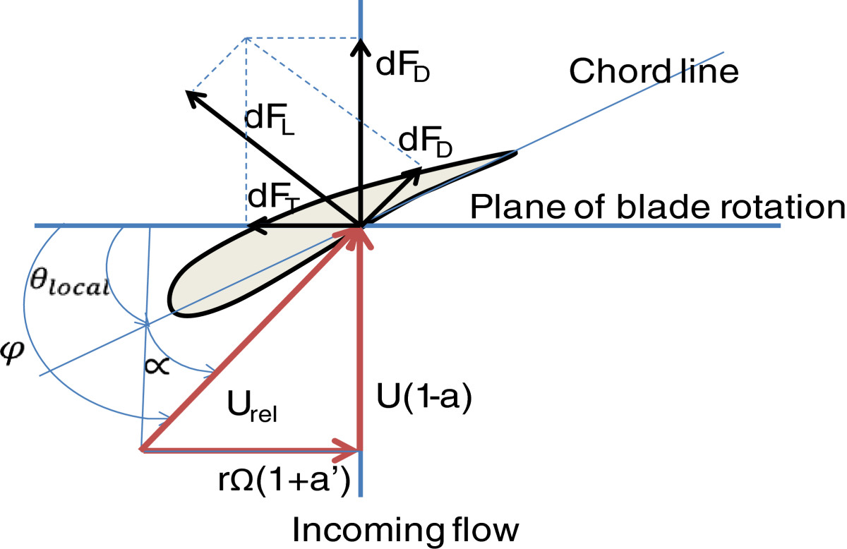
According to the blade element theory[ ¹¹ ] and by referring to Figure ¹ , one also has:

dT=σ′πρU21−a2sin2ϕC1cosϕ+Cdsinϕrdr

dQ=σ′πρU21−a2sin2ϕC1sinϕ−Cdcosϕr2dr

where σ ′ is the local solidity which can be calculated by σ ′ = Bc /2 πr ; here, B is the number of blades and c is the local blade chord length. φ is the angle of relative wind, C _l and C _d are the lift and drag coefficients, respectively.

Figure 1

Thus, the total torque at the shaft ( Q ) is the summation of dQ for all the blades elements, and the wind turbine power is given by P = Q * ω . Eventually, the wind turbine power prediction lies in solving the axial induction factor a and the tangential induction factor a ′[ ¹¹ ]. By combining Equations ¹ , ² , ³ , and 4, one can solve the induction factors a and a ′ as given below:

a=11+4sin2ϕσ′C1cosϕ+Cdsinϕ

a′=C1sinϕ−CdcosϕC1cosϕ+Cdsinϕλs+4λssin2ϕσ′ora′=aC1sinϕ−Cdcosϕc1cosϕ+Cdsinϕλs′

where λ _s is the local speed ratio which is defined as λ _s = ωr / U . The axial thrust coefficient C _T is expressed as:

CT=σ′1−a2C1cosϕ+Cdsinϕsin2ϕorCT=4a1−a

By substituting the two induction factors into Equation ² , the wind turbine performance can be assessed.

Corrections for BEM method

When the BEM method was originally developed by Glauert, it was far from giving accurate and reliable results before the implementation of some important corrections. These corrections include tip and hub losses, Glauert and Buhl empirical corrections, as well as the skewed wake correction in addition to the 3D rotational correction.

Tip and hub losses

Tip and hub losses consider the influence of vortices shed from the tip and hub, which play an important role in the induced velocity distribution at the rotor. Prandtl model is the most widely used model for calculating the tip and hub loss correction factors. An approximate formula for the Prandtl tip and hub function was firstly introduced by Glauert[ ⁴ ] as expressed below:

F=π2cos−1exp−f

Where f=BR−r2rsinϕ is for tip loss factor, and f=Br−Rhub2rsinϕ is for hub loss factor, where R is the radius of blade tip and R _hub is the radius of blade hub. Ultimately, the correction factor can be calculated by the multiple of the tip and hub loss correction factors, as illustrated in Equation ⁹ :

F=FtipFhub

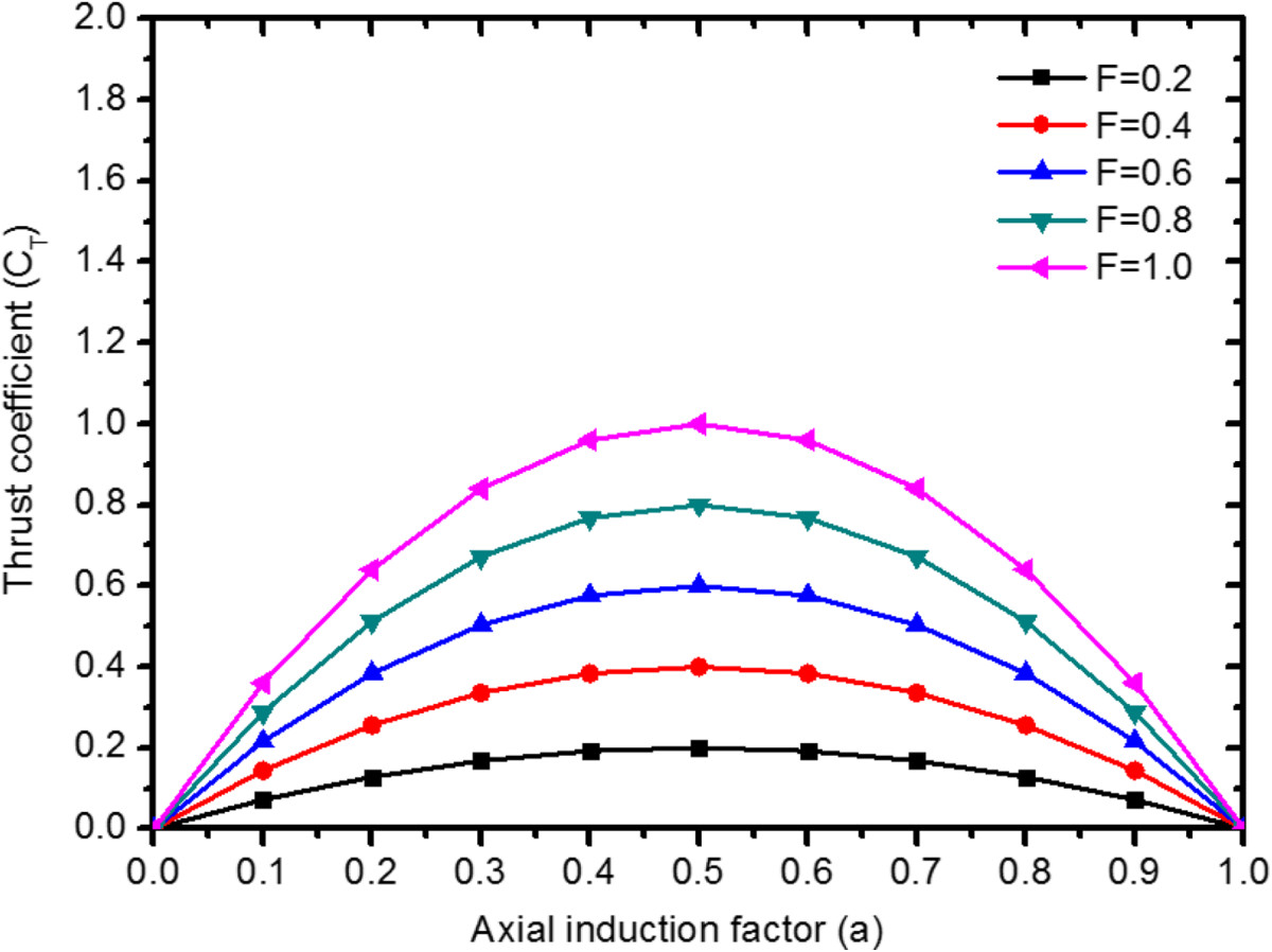
Figure ² shows the relationship between the thrust coefficient and axial induction factor at F ≤ 1 and with and without tip and hub correction factors. A pronounced increase in the axial thrust, observed as F , increases.

Figure 2

Due to the influence of the tip and hub correction factors, the forces derived from the momentum theory have to be modified accordingly:

dT=FρU24a1−aπrdr

dQ=4Fa'1−aρUπr3ωdr

Thus, the calculations for two induction factors and thrust coefficients are updated as follows:

a=11+4Fsin2ϕσ'Clcosϕ+Cdsinϕ

a'=Clsinϕ−CdcosϕClcosϕ+Cdsinϕλs+4λsFsin2ϕσ'ora'=aClsinϕ−CdcosϕClcosϕ+Cdsinϕλs

CT=σ'1−a2Clcosϕ+Cdsinϕsin2ϕorCT=4Fa1−a

Glauert and Buhl empirical corrections

As the induction factor is greater than 0.4, wind turbines will be under a turbulence wake. This puts an upper limit for the validity of the basic theory. Glauert developed a correction[ ¹² ] to the rotor thrust coefficient based on experimental measurements of helicopter rotors with large induced velocities. Buhl[ ⁸ ] later developed a new relation between rotor thrust coefficient and induction factor which solved the instability caused by applying Glauert correction as illustrated below:

a=18F−20−3CT50−36F+12F3F−436F−50forCT≥0.96

Figure ³ shows the Classical relationship between thrust coefficient and axial induction factor, Glauert correction relationship, Buhl empirical correction relationship, and experimental data of Moriarty et al.[ ⁶ ].

Figure 3

The widespread experimental data indicates that the thrust coefficient is not a simple function of axial induction factor in the turbulent wake region. As clearly shown from Figure ³ , the Buhl empirical relationship between C _T and a plausibly follows the experimental data trend and could also solve the instability/mismatch problem caused by Glauert's empirical relationship at the same time.

Skewed wake correction

Although BEM method was originally proposed to solve for the axisymmetric flow, wind turbines are often running at yaw angles. This again invalidates the basic theory unless a correction is used accounting for the skewed effect. Snel and Schepers[ ¹³ ] derived the following correction formulation:

askew=a1+15π32rRtanχ2cosψ

where χ is the wake skew angle, and ψ is the azimuth angle. However, Eggers's work[ ¹⁴ ] concluded that the correction can be large, emphasizing its inclusion.

Rotational effect

The effect of rotation was first investigated intensively for helicopter rotor. Later, the fact that aerodynamic power tends to exceed the design value for wind turbine starts attracting more attention and translated to different mechanisms. These include centrifugal pumping effect, stall delay, rotational augmentation, etc.[ ¹⁵ ]. Despite of these developments, a census approach is still lacking, particularly for the effect on the drag. Nevertheless, the 3D correction of Snel et al. received amble attention and is incorporated in present work. It provides an increase of the aerodynamic lift coefficient for the effects of rotation, which is described below:

cl,rot=cl,non−rot+3.1×λs21+λs2×cr2×cl,pot−cl,non−rot

where the ‘potential lift coefficient’ C _l,non−pot is defined as 2 π sin( ∝ − ∝ ₀ ), ∝ ₀ is the angle of attack when lift coefficient is zero.

Summarizing, the above mathematical formulation proposes an iterative procedure for solving the axial and tangential induction factors accounting for different types of losses. As obtaining the two induction factors is indispensable for predicting the performance of wind turbines, Figure ⁴ illustrates the flowchart for computing these induction factors.

Figure 4

The tolerance ( ε ) in the iterative procedures for the induction is set to be 0.001. The procedures are integrated to classical BEM method calculation, leading to the development of robust numerical procedures, i.e., extended BEM. The code follows the iterative procedure shown in Figure ⁴ . It provides the wind turbine power generation/coefficient as an ultimate result.

Verification of the extended BEM model

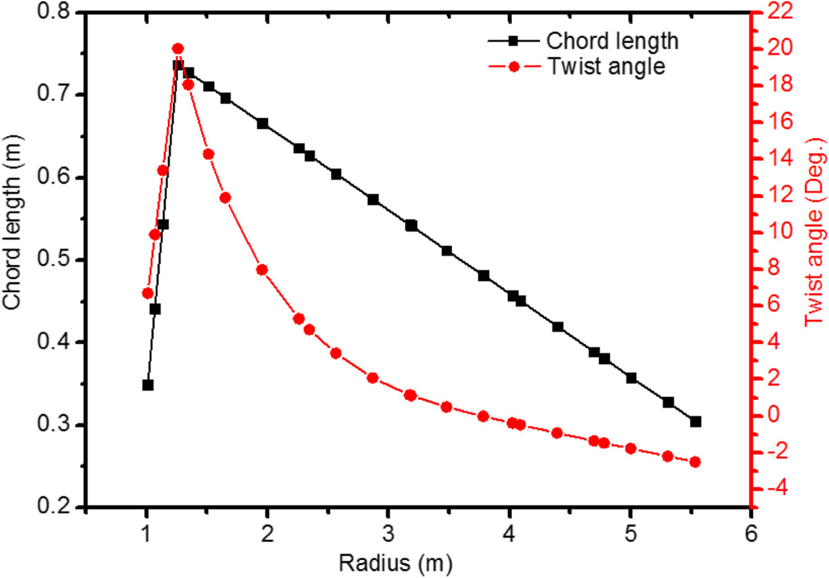
The UAE phase-VI turbine[ ¹⁶ ] is used as a baseline to validate the proposed extended BEM model. Its experimental data were collected by National Renewable Energy Laboratory (NREL) in the 24 × 36-m wind tunnel of NASA Ames. UAE phase-VI turbine is a two-bladed and S809 airfoil type wind turbine with fixed operation state of 72 RMP rotational speed and a three-degree pitch angle. The blades has a literal sweeping chord length of 0.737 m which decreases to 0.305 m and a twist angle of 20.04° at the largest chord[ ¹⁵ ] that fades to −2.50° at the tip, as depicted in Figure ⁵ .

Figure 5

The user of the code needs to provide the following necessary data: (1) the blade pitch angle, (2) sectional twist angle, (3) chord length at different radii, and (4) the lift and drag coefficients as a function of angle of attack. The aerodynamic data for S809 airfoil were taken from[ ¹⁵ , ¹⁷ ]. The airfoil aerodynamic data, as shown in Figure ⁶ , were initially developed at TU-Delft wind tunnel and subjected to the angle-of-attack shift technique for large angles of attack and empirical tool ‘stall coefficients (StC)’ for deep stall[ ¹⁵ ].

Figure 6

The influence of different corrections on the power coefficients of the turbine under different wind speeds were sought and compared with experimental data, as shown in Figure ⁷ .

Figure 7

It is clear from Figure ⁷ that the power coefficients obtained from BEM without any corrections overestimate the performance, while with tip and hub corrections, it reduces the performance at large margin. Simultaneously, the model with tip loss, Buhl empirical correction, and 3D correction of Snel et al. managed to predict the power coefficients under different wind speeds. However, the discrepancies between the results obtained from the model with tip loss and Buhl empirical correction and the experimental data can still be observed. As shown in Figure ⁷ , the results obtained from the model strictly follow the experimental data with slight underestimation. As this mismatch becomes large in other cases, it can be attributed to two reasons: (1) Empirical correction of the tip loss and Buhl require further improvements in order to describe wind turbine and incoming wind interaction and (2) lack of accuracy in the airfoil aerodynamic data that accounts for the rotation effect that will be inherited in the 3D correction.

Application of BEM on 3.5-kW HAWT

Windspot is a small size HAWT, 3.5-kW three-bladed turbine with a 4.05-m rotor diameter. It is characterized with low cut-in speed (<3m/s) and a rated power at 12m/s. It can be fitted with different set of blades, essentially at zero twist angle with a centrifugal/active pitch control system. The chord length is 0.254 m at the root, decreases linearly to 0.156 m at the blade tip.

Aerodynamic data

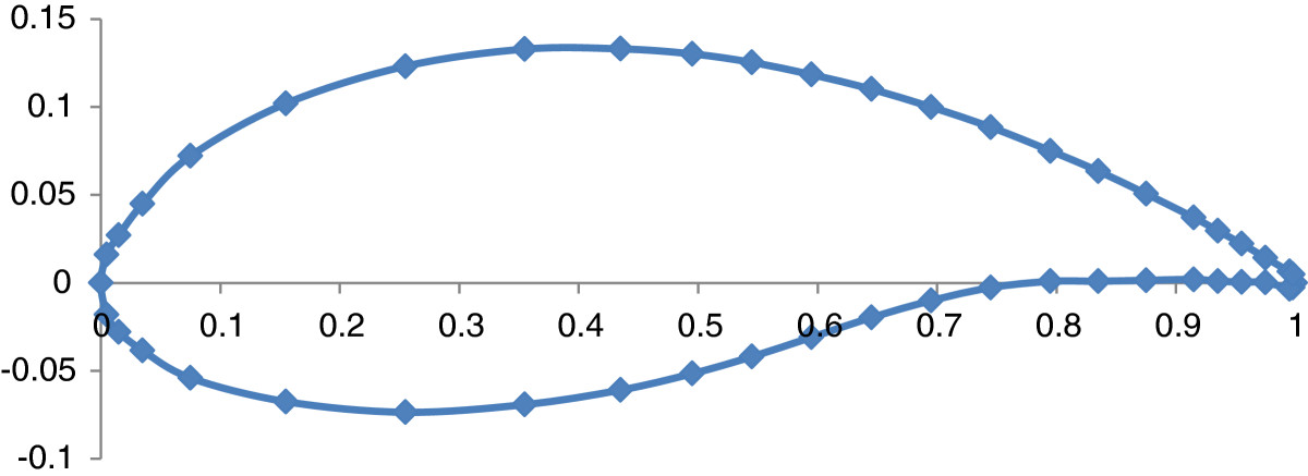
The Windspot airfoil was extracted from the solid model in the form of native IGES geometry. Panel method (governed by potential flow) and high fidelity CFD numerical simulations are developed and carried out to obtain the BEM required aerodynamic lift ( C _L ) and drag ( C _D ) coefficients at varying angle of attack. Figure ⁸ shows the geometry of the airfoil, in which the captured nodes divide the airfoil into several panels. The trailing and leading edges are further refined with additional panels.

Figure 8

Figure ⁹ shows the C _L result of the panel method which clearly varies linearly with the angle of attack. The panel solution is based on potential flow theory with no reference to the viscous boundary layer. These results, and when incorporated zero viscous drag, clearly will overestimate wind turbine performance.

Figure 9

High fidelity CFD simulation is also carried out for the Windspot airfoil. The flow is governed by the two dimensional, steady incompressible Navier–Stokes equations. These equations represent statements of mass and momentum conservation and are written after applying the scalar variable expansion ∅ix→,t=∅1¯x→,t+∅i′x→,t and ensemble (over bar) averaging as:

Continuity:∂ρ¯∂t+∂ρul¯∂xi=0

Momentum:∂ρul¯∂t+∂∂xjρu¯ju¯l=∂τij∂xj+ρ¯gi

Constitutive:τij=−p¯δij+μ∂ρul∂xj+∂ρuj∂xi−ρu′lu′j¯

where t is the time advancement, x _i is the Cartesian coordinate ( i = 1, 2), u _i is the velocity component in x _i direction, ρ is the density, g _i is the gravitational acceleration component in x _i direction, τ _ij is the stress tensor components, p is the pressure, μ is the molecular viscosity, u _i ^’ is the velocity fluctuations about ensemble average velocities. The ρu′lu′¯J term is the Reynolds stresses and is modeled utilizing the mean ( ū ) velocity via the common eddy viscosity k-epsilon turbulent. It is expressed as:

Turbulenceclosure:−ρu′lu′¯j=μt∂pu¯l∂xj+∂puj∂xi−23ρ¯kδij

where k is the kinetic energy u′ku′¯k and μ _t is the turbulent viscosity which links k and turbulent dissipation rate such that µt=fµCµρk2ε , where f _μ and C _μ are empirical constants. Substituting Equations ²¹ to ²⁰ conveniently allows summing the Reynolds stresses terms to the diffusion term (2nd right hand term in Equation ²⁰ ) with an equivalent viscosity μ _equ = μ + μ _t . Therefore, closure of the above system is achieved with the integration of two additional transport equations for k and ε . The above equations are discretized on well-posed/bounded domain, forming an algebraic system of equations. The boundary conditions including incoming velocity (Dirichlet), side boundaries symmetry (Neumann), outflow at the exit, and no-penetration, no-slip at the airfoil surface.

The airfoil geometry and the flow zone model were built and discretized using quad-type cells. The airfoil surface is padded with a refined cell cluster of less than 0.01% chord length initial height and at smooth growth of 1.4 to achieve one unit normalized wall distance ( y + = 1). The geometry, the baseline mesh, and the imposed boundary conditions are shown in Figure ¹⁰ . The domain was subjected to the upstream uniform velocity (5 m/s which is the annual average wind speed in Masdar City[ ¹⁸ ]) and the output atmospheric pressure to be used during the iteration in the event of recirculation at the outflow boundary.

Figure 10

Results and discussion

The Fluent iteration, double precision, and pressure-based SIMPLE solver were used to compute the aerodynamic data as a function of angle of attack with as low as 10 ⁻¹⁰ residuals in the continuity and the two momentum equations. Except for the pressure, a second order discretization is implemented. Mesh sensitivity studies were carried out first to assess solution dependency. Results of the 5° angle of attack case is carried out at the baseline, fine and two levels of coarseness, and these are summarized in Table ¹ .

The mesh dependency of the solution was observed to reduce as it became finer. The baseline mesh appears to capture the solution at a reasonable level of accuracy relative to the other successive refinement and coarseness. This is also clear from the normalized value of the wall ( y +) which is desired to be one unit to avoid excessive refinement. Figure ¹¹ shows the results of the lift and drag coefficients as functions of the angle of attack for the 3.5-kW Windspot airfoil from baseline mesh. The data is fitted with an appropriate polynomial for convenient integration in the BEM code.

Figure 11

The improved BEM is used to estimate the Windspot power coefficient, which is limited by Betz Law (<0.59)[ ¹⁹ ]. As the operation of the wind turbine is unknown, it is reasonably assumed to operate at a fixed rotational speed of 12 rad/s and 7° pitch angle. The power coefficients under different wind speeds, yet at that fixed rotational speed, are obtained and compared to experimental data[ ²⁰ ], as depicted in Figure ¹² . Results of the simulation show appreciable deviation from those obtained experimentally while continue to exhibit a plausible trend.

Figure 12

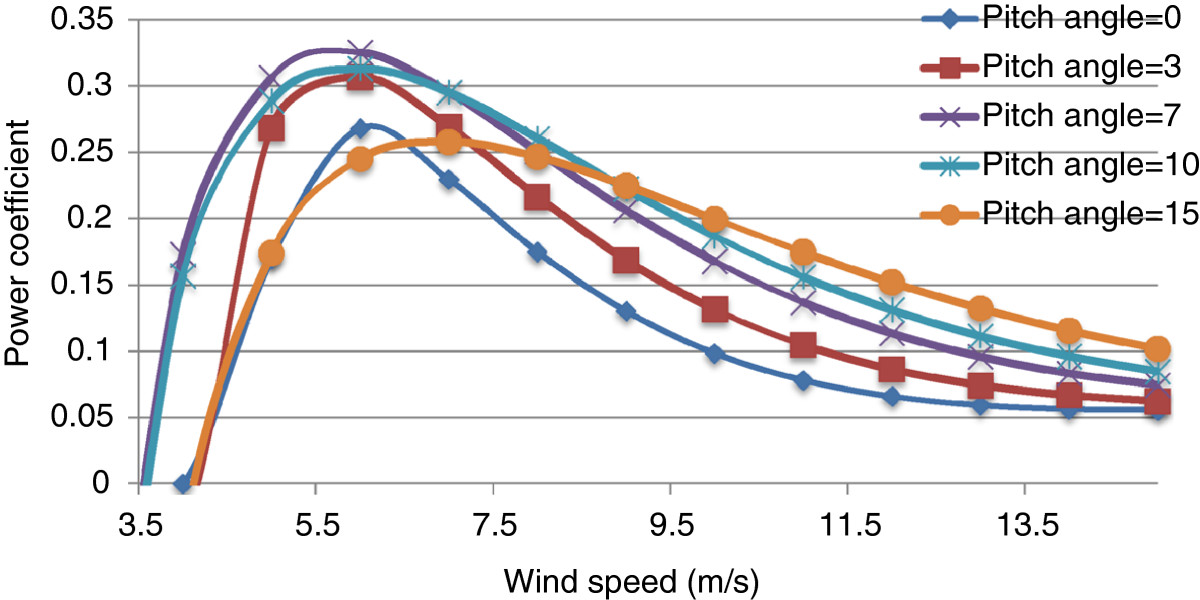
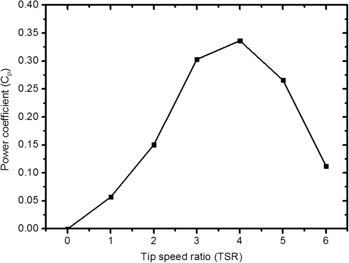
The influence of the pitch angle, twist angle, and TSR is also investigated. Figure ¹³ shows the effect of different pitch angles at a zero twist at the previously considered rotational speed (12 rad/s). A pitch angle in the range of {3,7} appears to be more optimal for a flow speed up to 8 m/s. Figure ¹⁴ depicts the influence of the twist and clearly shows that a 10° twist can lead to a measurable increase in the power coefficient which translates to a measurable increase (up to 4°) in the overall angle of attack. Higher twist resulted in near stall condition and drastic fall in the power coefficients. The influence of the tip speed ratio is also investigated at the optimal pitch and twist angles to observe their combined effect on the power coefficient as shown in Figure ¹⁵ .The tip speed is varying here by the rotational speed. The results suggest that a maximum power can be obtained near TSR of 4.

Figure 13

Figure 14

Figure 15

The wind turbine is under different operational conditions which are listed in Table ² . It is clear from Figures ¹³ and ¹⁴ that choosing a proper pitch angle and designing a blade with proper twist angle are important for wind turbines. Excessive choice of pitch angle combined with twist would also lower the harvested wind turbine energy. Figure ¹⁵ shows that TSR as another important parameter for wind turbine, and higher power coefficients is achieved by operating at a suitable TSR value.

Conclusion

An improved BEM code for HAWT is developed. It is incorporating four important corrections: (1) tip loss, (2) Buhl empirical correction, and (3) skewed wake correction, as well as (4) 3D correction of Snel et al. These corrections extend the application of the BEM method to the turbulent wake regime of the HAWT. The developed code was validated by comparing the results from the code against those of NREL measured data of the UAE phase-VI turbine. The accuracy of the BEM inherently depends on obtaining an accurate aerodynamic data, i.e., lift and drag coefficient as a function of angle of attack. Therefore, potential theory (via Panel method) cannot sufficiently provide such data. Furthermore, as wind turbine airfoil shapes depart from classical NACA series, high fidelity CFD analysis for turbine blade was carried out. Results of the calculation that were based on the extended BEM show a plausibly match with the experimental trend of the Windspot turbine. Furthermore, detailed performance assessment was carried out by considering the effect of the twist angle, pitch angle, and TSR. The code illustrated these effects and results show designing blades with proper twist angle that harmonized with suitable TSR and pitch angle can definitely lead to substantial gain in performance of over 10%. In the case of 3.5-kW Windspot, revising the blade with 0 to 10-degree twist angle and operating the wind turbine under 7-degree pitch angle and TSR around 4 can lead to significant increase in power generation.

Authors' information

IJ is currently an associate professor at Masdar Institute of Science and Technology. Before, he worked as a visiting ME professor at MIT. He also possesses extensive industrial experience of over 12 years in aerospace and automotive from Michelin and GE. SL is currently a doctorate degree student.

References

Janajreh et al. (2010) Aerodynamic flow simulation of wind turbine: downwind versus upwind configuration (pp. 1656-1663) 10.1016/j.enconman.2009.12.013
Janajreh et al. (2010) Numerical simulation of tower rotor interaction for downwind wind turbine
Hu et al. (2006) A study on stall-delay for horizontal axis wind turbine (pp. 821-836) 10.1016/j.renene.2005.05.002